Results of theoretical and experimental studies of solar wind and active galactic nuclei on LFVN VLBI network using S2 recording system
V. G. Gavrilenko1, M. B. Nechaeva2, A. B.Pushkarev3,4, I. E. Molotov3,5,6,7, G.Tuccari8, A. S. Chebotarev9, Yu. N. Gorshenkov9, V. A. Samodurov10, X. Hong11, J. Quick12, S.Dougherty13 and S. Ananthakrishnan14
1 N. I. Lobachevsky State University of Nizhny Novgorod, Nizhny Novgorod, Russia; 2 Radiophysical Research Institute, Nizhny Novgorod, Russia; 3 Central Astronomical Observatory, St. Petersburg, Russia; 4 Scientific Research institute "Crimean Astrophysical Observatory," Nauchny, Crimea, Ukraine; 5 Central Research Institute for Machine Building, Korolev, Moscow Region, Russia; 6 Keldysh Institute for Applied Mathematics, Moscow, Russia; 7 JSC "Vympel" Interstate Corporation, Moscow, Russia; 8 Istituto di Radioastronomia, Noto, Italia; 9 Special Design Bureau of Moscow Power Engineering Institute, Moscow, Russia; 10 Pushchino Radio Astronomy Observatory of Lebedev Physical Institute, RAS, Puschino, Russia; 11 Shanghai Astronomical Observatory, Shanghai, China; 12 Hartebeesthoek Radio Astronomy Observatory, Hartebeesthoek, South Africa; 13 Dominion Radio Astrophysical Observatory, Pentictone, Canada; 14 National Centre for Radio Astrophysics of Tata Institute of Fundamental Reseach, Pune, India.
We discuss the results of two sessions of observations at the Low-Frequency VLBI Network (LFVN), carried out in 1999 (INTAS99.4) and 2000 (INTAS00.3) at a wavelength of 18 cm using the S2 recording system and processed using the correlator system in Pentictone, Canada. In different configurations of the experiments on studying the solar wind and active galactic nuclei, the antennas at the following sites were employed: Medvezhji Ozera (RT-64, Special Engineering Bureau of Moscow Power Engineering Institute, Russia), Pushchino (RT-22, Pushchino Radio Astronomy Observatory, Russia), Hartebeesthoek (RT-25, South Africa), Noto (RT-32, Italy), Shanghai (RT-25, China), Pune (RT-45, India), Svetloe (RT-32, Institute of Applied Astronomy RAS, Russia). The work resulted in successful testing of the method of radio probing of the solar-wind plasma by radiation of extragalactic sources, supplemented with the method of radio interferometric reception. Spectral analysis of the obtained data allowed us to estimate the index of spatial spectrum of the electron number density fluctuations and the transfer velocity of the solar-wind inhomogeneities on the sounding path. We present and discuss the retrieved images of STA-102 quasar and the BL Lacertae object 1418+546 with millisecond angular resolution and demonstrate the results of modeling the structure of these sources.
1. INTRODUCTION
Transition of worldwide radio-interferometer networks with very long bases (VLBI) to the use of wideband recording terminals of radio-astronomical data (MARK-III, VLBA, and K-3) made participation of most Russian radio telescopes in international VLBI experiments impossible. Therefore, a pilot project on creating the international low-frequency VLBI network (LFVN) was started in 1996 under support of INTAS (project No. 96-0183). The largest Russian, Ukrainian, and Indian radio telescopes joined the project [1, 2]. As one of directions for LFVN operation, opportunities of organization of a subsystem of radio telescopes equipped by S2 recorder [3] were studied. This Canadian VLBI terminal exceeded MARK-III and K-3 by its capabilities and ensured the recording of digital data with 1- or 2-bit digitization at eight home video recorders using 16 channels with a total speed of up to 128 Mbit/s (equivalent recording bandwidth to 64 MHz), but was several times cheaper. Moreover, there was positive experience of work with this recorder: the first transcontinental experiment at a wavelength of 18 cm with the use of the S2 recorder and participation of the Russian RT-70 site "Ussuriisk" and RT-64 site "Parks" and RT-26 site "Hobart" (Australia) was held in November 1993. Primary data processing was carried out using ATNF (The Australian Telescope National Facility) correlator in Sydney (Australia). Secondary processing aimed at studies of OH masers was performed at Astro-Space Center of the Lebedev Physical Institute (ASC LPI) [4] and ATNF. The second testing experiment was held in June 1996 with the base between RT-64 in Medvezhji Ozera (Russia) and the Australian DSN (Deep Space Network) RT-70 site in Tidbinbilla. In that case, the largest baseline length of 11538 km for the S2 recorder was achieved, which was close to the theoretical limit of ground-based VLBI bases. The main correlation processing of experimental data was carried out at ATNF. The obtained results were published in [5]. These experiments demonstrated the operational integrity of the international VLBI network based on the use of S2 recorder. The purchase of four S2 terminals by the ASC LPI in 1998 allowed us to begin its full-scale implementation within the framework of the LFVN project. By that time, the Canadian recorder already got wide adoption in Russia (three S2 were purchased by the Institute of Applied Astronomy RAS in 1994) and abroad (S2 were bought by Australia, China, India, and USA; additionally, Canadian Space Agency installed several terminals at key radio telescopes in the world within the framework of the VSOP project). A new 6-station S2 correlator in Pentictone (Canada) began operation [6].
The first two S2 terminals of ASC LPI were installed at RT-22 and RT-64 radio telescopes in Pushchino and Medvezhji Ozera, respectively, since these telescopes were equipped by radio receivers tuned to the wavelength 18 cm, necessary video converters, and S2 interfaces. In August 1998, a testing observation session was carried out with the use of the INTAS98.2 S2 recorder (recording bandwidth 2 MHz, from 1664.99 to 1666.99 MHz). RT-64 (Medvezhji Ozera, Russia), RT-43 (Green Bank, USA), and RT-26 (Hartebeesthoek, South Africa) sites participated in that session. The data recorded onto magnetic tapes were successfully processed in Pentictone, and after that, a cooperation agreement on organization of LFVN experiments was signed between DRAO (Dominion Radio Astrophysical Observatory) and ASC LPI. The results of studies of quasars and solar wind, carried out using the LFVN with S2 recorder, are described in this paper. From 2002, the processing of astrophysical VLBI observations in Pentictone was stopped because of the end of the VSOP project, which prevented the further development of the LFVN S2 subsystem. The data of the experiment organized at the beginning of 2003 were not processed.
2. OBSERVATIONS AND PROCESSING
The first official experiment using the INTAS98.5 S2 subsystem (two 2-MHz bands, 1664.99-1666.99 MHz and 1666.99-1668 .99 MHz) was held from November 30 to December 2, 1998 with participation of six sites, i.e., RT-64 (Medvezhji Ozera, Russia), RT-22 (Pushchino, Russia), RT-300 (Arecibo, USA), RT-32 (Svetloe, Russia), RT-43 (Green Bank, USA), and RT-26 (Hartebeesthoek, South Africa). The VLBI responses for bases including the radio telescopes in Svetloe and Pushchino, equipped by S2 recorders, were obtained for the first time. Using the results of the experiment with participation of three Russian sites, images of quasars were built for the first time using the LFVN [7]. In 1999, the RT-25 radio telescope of the Shanghai Astronomical Observatory (China) joined the project. The S2 terminal was also installed at the RT-32 radio telescope in Noto (Italy), which participated earlier in LFVN observations with the use of a MARK-II terminal. During the period from November 29 to December 2, 1999, the IN-TAS99.4 experiment was carried out. The sites in Medvezhji Ozera, Pushchino, Svetloe, Noto, Shanghai, and Hartebeesthoek participated in the observations. The total duration of the experiment was 43 h. The measurement data were successfully processed in Pentictone with an averaging time of 2 s. The bandwidth was 4 MHz (1664.99-1668 .99 MHz) for 256 spectral bands of 15.625 kHz each. For solar-wind studies, the correlation of data was performed using the 0.1-s averaging time. The results were partially published in [8] and also presented below. The next experiment INTAS00.3 was carried out during the period from November 28 to December 1, 2000. The total duration of the experiment was 50 h. Besides the radio telescopes in Medvezhji Ozera, Pushchino, Noto, Shanghai, and Hartebeesthoek, the 45-m antenna of GMRT (Giant Meterwave Radio Telescope) system in India was employed in the experiment. For this purpose, a 4-channel S2 interface ensuring the connection of the S2 terminal to a video converter was built for the NCRA TIFR institute. An expedition of Russian scientists was sent to Pune for the time of preparing and performing the session. These observations were the first ones performed at GMRT at a wavelength of 18 cm with signal recording in the 8-MHz bandwidth (1664.99-1672.99 MHz). The data were processed in Pentictone using 256 spectral channels of 31.25 kHz each and 2-s averaging time. All the experiments, i.e., INTAS98.2, IN-TAS98.5, INTAS99.4, and INTAS00.4, were carried out using the left-hand circular polarization of radiation and one-bit signal digitization. Some parameters of radio telescopes (the diameter, the system temperature Tsys, and the equivalent system flux density SEFD) are presented in Table 1.
TABLE 1. Diameters of antennas and their characteristics at a frequency of 1.66 GHz.
Antenna
Diameter, m
Tsys, K
SEFD, Jy
Medvezhji Ozera, Russia
64
65
110
Pushchino, Russia
22
111
1590
GMRT, India (2000)
45
70
290
Hartebeesthoek, South Africa
26
50
530
Noto, Italy
32
105
1020
Shanghai, China
25
78
980
Svetloe, Russia (1999)
32
71
394
The use of the Hartebeesthoek antenna significantly increased the angular resolution in the North-South direction. The maximum-projection length of the base reached 10170 km for Shanghai and Hartebeesthoek sites. To build the radio image, 5-8 observations with a mean duration of 30 min were performed for each source. For the part related to the diagnostics of solar-wind plasma, the near-solar space with the established solar-wind flow was studied [9]. For this purpose, the sources located at angular distances from 8° to 51° from the Sun were observed. These were mainly point sources, i.e., unresolved for the used bases, or symmetric ones. To exclude the influence of the Earth's atmosphere on the interferometer signal, only the time intervals for which the sources for most antennas were located at elevation angles above 15° were chosen.
3. STUDIES OF ACTIVE GALACTIC NUCLEI
In the INTAS00.3 experiment, several extragalactic sources were observed. For two of these sources (1418+546 and CTA 102), radio images were built and the structure for decaparsec scales was analyzed. Editing and calibration of VLBI data (see [10] for detail) were carried out using the AIPS software developed at NRAO (National Radio Astronomy Observatory, Soccoro, USA) and employing standard techniques. For amplitude calibration, the amplification curves and system temperatures measured for each antenna participating in observations were used. Primary phase calibration was performed using the AIPS FRING procedure with a coherent integration time of 120 s and the subsequent phase correction to compensate for the residual delay by the entire time of experiment. The telescope in Medvezhji Ozera was used as the reference antenna. Retrieval of radio images by the hybrid-mapping method was performed using the DIFMAP package [11]. For hybrid mapping, a model of a point source in the phase center was used as the initial model for each source. The convergence was reached on average for 20 iterations including the phase and phase-amplitude self-calibrations. When building the final source map, the natural weighting of the visibility-function values was used.
TABLE 2. Source models.
Source
α, h:min:s
β deg:arc min: arc s
Component
Flux, Jy
r, 10-3 arc s
φ, deg
FWHM, 10-3 arc s
1418+546
14:19:46.597
+54:23:14.787
C
0.74
-
-
0.32
J1
0.34
1.42
127
0.23
J2
0.08
2.29
116
0.26
CTA 102
22:32:36.408
+11:43:50.904
C
2.37
-
-
1.15
J1
0.41
7.23
145
1.64
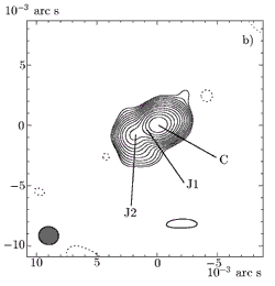
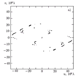
On the images shown below, solid and dashed lines show the isocontours of the positive and negative flux densities, respectively. The isocontours are plotted with a √2 step. The synthesized antenna pattern is shown in the lower left corner of each map. The scales of the vertical and horizontal axes are given in arc milliseconds. In the figures showing the filing of the spatial-frequency plane (the uv-plane), the scales of the vertical and horizontal axes are given in millions of wavelengths (λ = 18 cm).
The source structure was modeled on the basis of the circular Gaussian components by comparing the model with fully calibrated observation data on the (u, v) plane of spatial frequencies using DIFMAP. The source models are presented in Table 2. The object names are given in the first column, the equatorial coordinates for the year 2000 epoch, in the second and third columns, the component identifiers, in the fourth column, the integral radiation flax of the model component, in the fifth column, the component location on the map in polar coordinates r and
3.1. The source 1418+546
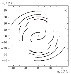
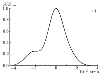
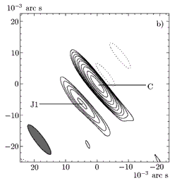
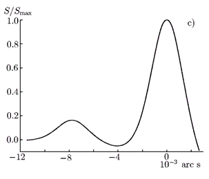
The source 1418+546 is the BL Lacetrae object and is located at the center of the parent galaxy which can be attributed to the spiral type SO by its surface-brightness profile [12]. This happens very rarely, since most parent galaxies of the Lacertae objects are elliptic. The object's red shift z = 0.152 was measured by Stickel et al. [13] by both absorption lines of the parent galaxy and the emission lines of O II (λ = 3727 A) and O III (λ = 4959 A and 5007 A) [14]. Figure la shows the filing of the spatial-frequency plane for the 1418+546 source obtained from the data of INTAS00.3 observation session at the wavelength λ = 18 cm. Figure 1b shows the VLBI map (retrieved brightness distribution) of this object with a visible intensity peak of 797 mJy in a beam. The lower contour is plotted at 3.25% of the maximum level. The size of the main beam of the synthesized antenna pattern used for the image retrieval equals 1.7 x 1.5 arc ms, and the position angle of the larger axis is 82°. The results of modeling of the source structure are shown in Table 2. Figure 1c shows the linear brightness distribution with a position angle of 116°, normalized to the maximum value of the radiation flux density.
Fig. 1
The VLBI map of this object shows a one-sided (due to the Doppler brightening) structure of the core-jet type in the South-East direction with a position angle of about 120°. The jet propagates to an angular distance 3.2 arc ms from the core. To pass to the linear scale, we use the following arguments. If the Universe expansion is taken into account, then the angular scale θ is related to the linear scale L as
where c is the speed of light in vacuum, H is the Hubble constant, q0 is the slow-down parameter, and z is the red shift. If we measure L and θ in parsecs and arc milliseconds, respectively, and use the standard Friedman model of the Universe with the slow-down parameter q0 = 0.5 and the Hubble constant H = 70 km/(s ∙ Mpc), then we obtain
Thus, for the 1418+546 source with the red shift z = 0.152, the angular distance of 3.2 arc ms corresponds to 7.9 pc on the linear scale in the image-plane projection.
For a model of a homogeneous spherical source [15], the brightness temperature of radiation from the VLBI-core region (By the VLBI-core we mean the most compact structure component with optical depth about unity) in the source reference frame is calculated as
where Score is the flux density of the VLBI-core of the object, Θ is the angular size of a circular Gaussian component corresponding to the VLBI core at the half-power level (the FWHM parameter in Table 2), v is the frequency of observation, k is the Boltzmann constant, and z is the red shift. In this case, if we measure Score, Θ, and the frequency of observation v in Jy, arc ms, and GHz, then we have
Using the data of Table 2, we obtain that the brightness temperature of the 1418+546 object is 1.33 ∙ 1012 K, which exceeds the theoretical value of 1011 K for the brightness temperature for the case of energy equipartition [16] and also exceeds the inverse Compton-effect limit of 1012 K [17]. It can be explained by Doppler brightening which is a consequence of the directivity of relativistic-jet radiation, i.e., the smallness of the angle between the line of sight and the direction of the jet velocity.
3.2. The source CTA 102
The object CTA 102 (2230+114) is attributed to the class of strongly polarized quasars and is the first source in which the variability in the radio-frequency range was found [18]. The optical spectrum of this object has a strong emission Mg II line λ = 2798 A with the red shift z = 1.037 [19]. The structure of CTA 102 on kiloparsec scales is the dominating core and two components [20], located at distances of 1.6 and 1.0 arc s with position angles of about 140° and -40°, respectively.
Figure 2a shows the uv-plane for the CTA-102 source at a wavelength of 18 cm. Figure 2b shows the VLBI map of this object at a frequency of 1.66 GHz with a maximum flux density of 2490 mJy in a beam. The lower contour is plotted at a level of 5.02% of the maximum. The size of the main lobe of the synthesized antenna pattern, used for the image retrieval, is 11.9 x 2.9 arc ms, and the position angle of the larger axis is 37°. In Fig. 2c, the linear brightness distribution with a position angle of 145°, normalized to the maximum value of the flux density, is shown.
Fig. 2
The VLBI structure of the source 2230+114 consists of a bright core and a jet. The jet propagates to the South-East with a position angle of 145° to an angular distance of 3 ms (18.3 pc in the linear scale as projected onto the image plane). The modeling results for the source structure are presented in Table 2. The brightness temperature of CTA 102 was 5.9 ∙ 1011 K.
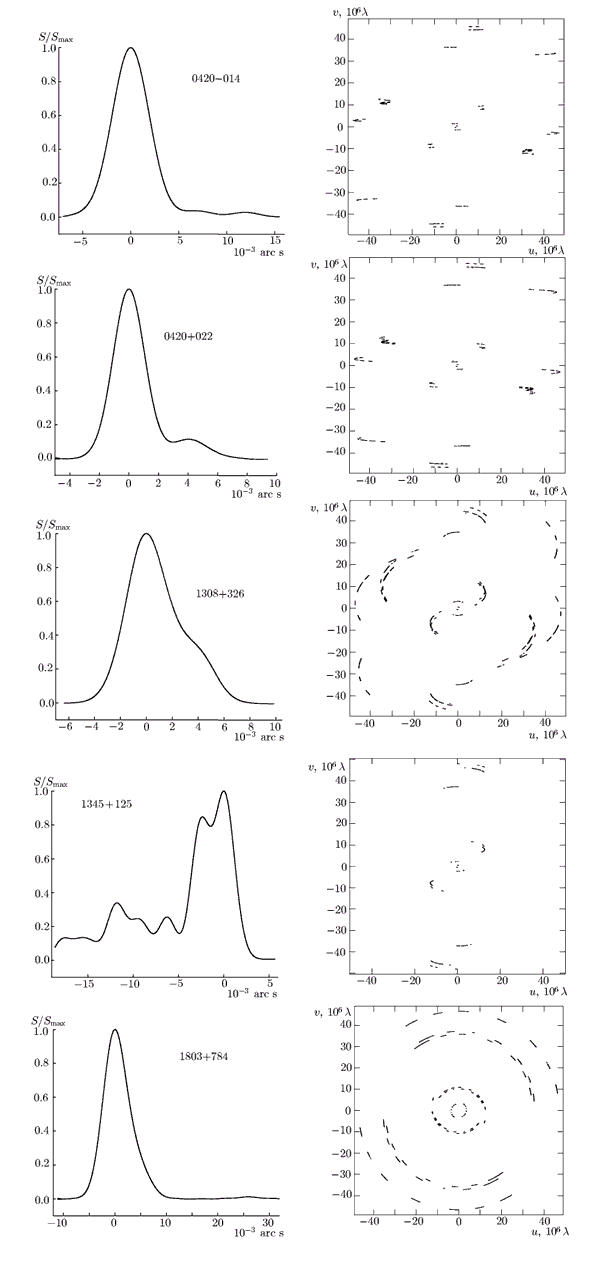
For active galactic nuclei observed in the experiment of the year 1999, the radio-brightness maps were plotted and modeling of their structure was carried out [8]. In this paper, we present the linear brightness distributions for the sources 0420-014, 0420+022, 1308+326, 1345+125, and 1803+784 along the directions of jets with position angles 4°, 90°, -58°, 152°, and -105°, normalized to the maximum values of the radiation flax density equal to 1337, 770, 1576, 582, and 1482 mJy, respectively (Fig. 3, left), and the obtained filings of the uv-planes (Fig. 3, right). In all cases except for the 1345+125 source, the quality of the filing of the spatial-frequency plane can be considered satisfactory, since in the experiment small, mid, and long bases were realized. However, it is extremely important to increase the number of network sites participating in the observations for improving the dynamic range of the maps and increasing their reliability.
Fig. 3
4. EXPERIMENTS ON RADIO RAYING OF SOLAR WIND
4.1. Theory
At present the interplanetary and near-solar plasmas are diagnosed by various radio astronomical means based on the radio-raying technique [9]. A prospective direction in this field of studies is supplementing the traditional radio-raying method by the interferometry method [5, 21]. In [22, 23], the application of radio interferometric methods for diagnostics of a turbulent nonstationary medium was considered in detail. We solved both the direct and inverse problems, i.e., analyzed the electromagnetic-wave propagation in an inhomogeneous medium and its influence on the device output signal and considered the means for retrieving information on the medium of propagation from the spectral composition of the interferometer signal. We analyzed the power spectrum of fluctuations of the VLBI response to the noise-like source radiation passed through a turbulent solar-wind plasma. As the continuation of these studies, specific cases of the influence of strong and weak fluctuations of a medium parameter on the interferometer signal were analyzed numerically. On the basis of the obtained methodic recommendations, we analyzed the results of VLBI experiments INTAS99.4 and INTAS00.3 on radio-raying of the solar-wind plasma.
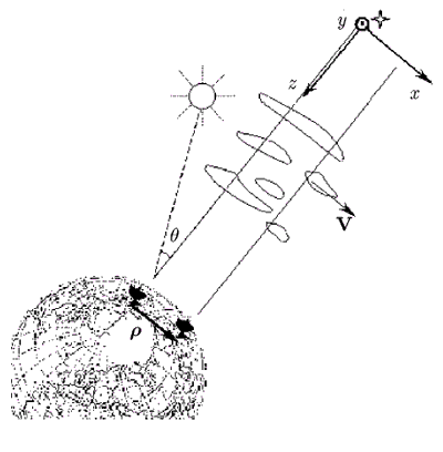
The experiments were performed according to the following scheme. The radiation of a distant source in the form of a quasi-plane wave propagates along the z axis through a turbulent medium with large-scale random irregularities of the electron density and is received by a two-element multiplicative interferometer with the base ρ in the xy plane perpendicular to the propagation direction (Fig. 4).
Fig. 4
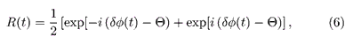
The signals received by two antennas are multiplied at the same time moment t. As a result of this procedure carried out in the correlator, the fluctuating difference of the signal phases at two receiving sites is found. We represent the output signal of the complex correlator [10] as
where δφ(t) is the difference in the phase fluctuations of the signals received by different antennas at the same time moment, and Ω is the additional constant phase shift introduced into the correlator signal. Such a procedure has several advantages compared with the traditional single-site reception, since it allows one to study the field fluctuations introduced only by the turbulent medium at two propagation paths. In this case, the influence of the fluctuations of the own source radiation is excluded, which makes it possible to study the medium upon its raying by not only monochromatic signals from spacecraft, but also wide-band noise-like signals of a natural radio source.
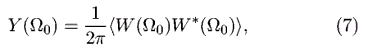
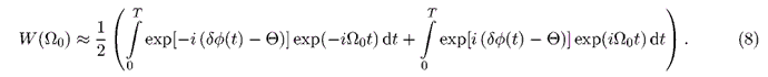
Then, a spectral analysis of the interferometer signal was performed. For a large sample duration (T -> ∞), the signal power spectrum is expressed as follows [24]:
where the angular brackets denote statistical averaging, and
Experimental frequency spectra (7) obtained by the method described above and being the most important statistical characteristic of a signal were analyzed for retrieving information on the medium of propagation.
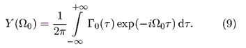
We represent the power spectrum as the Fourier transform of the autocorrelation function Г0(τ) of the correlator signal R(τ):
The function Г0(τ) in Eq. (9) is the fourth-order coherence function for the complex fields in the reception sites [22, 23] and, taking Eq. (8) into account, can be represented as
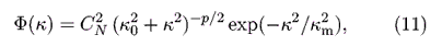
The field fluctuations were described using the geometrical-optics method. The medium characteristic that was studied was the electron number density of the solar-wind plasma. To describe temporal variations in the parameters of the solar-corona medium, the frozen-in hypothesis valid at distances R > 15RΟ from the Sun, where RΟ is the solar radius [9], was used, i.e., it was assumed that the electron-density inhomogeneities do not vary in time and move radially from the Sun with velocity V equal to the solar-wind velocity. The spatial spectrum of electron-density fluctuations was specified by a power-law function with the index p in the wave-number interval κ є [κ0,κm], where κ0 = 2π/Λ0, κm = 2π/l0, Λ0 and l0 are the outer and inner turbulence scales, respectively [25]:
where C2N - is the structure coefficient characterizing the intensity of electron-density fluctuations
Here, σ2N is the variance of the electron-density fluctuations, and Г(x) is the gamma function. It is assumed that such a shape of the power-law spectrum satisfactorily describes the distribution of the electron-density fluctuations in the solar-wind region at angular distances above 2° in the decimeter range of wavelengths [25].
The above-mentioned approximations used in the theoretical analysis of the interferometer signal allowed us to simplify calculations and obtain the expressions for the interference-signal spectrum which contain information on the medium of propagation, such as the solar-wind speed, the spatial distribution of electron number density in the sounded region, the intensity of density fluctuations, etc. However, the retrieval of this information from experimental spectra is difficult, since the spectrum calculated by Eq. (9) is a complex combination of separate integral parameters of the turbulent medium. To calculate the perturbations of the interferometer signal caused by the propagation medium and estimate some of its characteristics, we consider the limiting cases of the radiation propagation through weak and strong perturbations.
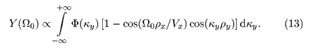
In the case of weak phase fluctuations, the power spectrum of the interferometer signal is that of the random phase difference of the signal at two reception points. For Θ = π/2, the power spectrum of the interferometer signal has the form [23]
Here, ρ^ = (ρx,ρy) and V^ = (Vx, Vy) are the projections of the interferometer base vector and the medium velocity onto the plane perpendicular to the radiation direction. When deriving Eq. (13), it was assumed that the x axis of the coordinate system is parallel to the vector of the medium velocity, i.e., Vy = 0.
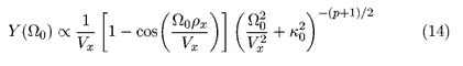
In the case where the interferometer base is predominantly directed along the drift velocity of the medium inhomogeneities (ρ^ = (ρx,0), V^ = (Vx, 0)), the power spectrum is described by a simple formula
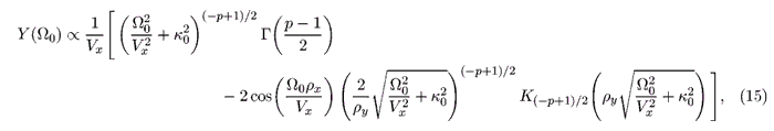
For an arbitrary relative orientation of the vectors of the interferometer base and the medium velocity, where the condition ρ^||V^ is violated, Eq. (13) for the spectrum can be transformed to
where K(-p+1/2)(x) is a modified Bessel function of the second kind.
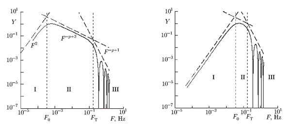
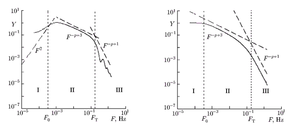
Let us analyze the shape of the power-spectrum envelope for weak phase perturbations. We construct various approximations of the function Y(F] for three frequency ranges:
In Eq. (16) and below, F = Ω0/(2π).
Function (14), valid for ρ^||V^, is plotted in Fig. 5. Dashed lines show the curves Y1, Y2, and Y3, corresponding to the spectrum envelope in the three frequency ranges specified in Eq. (16). The power spectrum has a clearly pronounced main maximum whose frequency Fmax, according to the adopted model of a turbulent flow in the solar wind, is determined by the index p of the spatial spectrum of electron-density fluctuations, the drift velocity V^ of inhomogeneities, and the outer turbulence scale Λ0:
(in this case, V^ = Vx).
Although the frequency Fmax is related by a simple expression with the medium parameters, it is impossible to diagnose the solar-wind plasma by this characteristic point of the spectrum. Since spatial spectum (11) of the number-density fluctuations is defined at the interval of wave numbers κ0 < κ < κm, the obtained formulas (13)-(16) for the spectrum of interferometer response are valid for frequencies above the characteristic frequency F0 = V^/Λ0 [25]. As follows from Eq. (17), the main-maximum frequency is comparable with F0: for example, for the index p = 11/3 corresponding to the Kolmogorov turbulence model [25], Fmax = √3F0. Hence, the estimates of the medium parameters in the range of the main spectral maximum can prove unreliable. Therefore, it is suggested to use the higher-frequency part of the spectrum for which model (14)-(15) works more reliably to obtain the medium parameters.
The spectral index of the curves Y2 and Y3 for the frequency intervals II and III is unambiguously related to the index p of spatial spectrum of the electron-density fluctuations (see Eq. (11)), which allows one to obtain this parameter from the experimentally measured spectra.
It is noteworthy that the spectrum shape with a smooth decrease in the interval II is observed only for a sufficiently large outer turbulence scale Λ0. For small Λ0, the interval II is significantly shortened, while the main maximum is shifted to the higher-frequency range. When calculating the function shown in Fig. 5, Λ0 was assumed equal to 106 km, which corresponds to the developed turbulent processes in the solar wind [9]. The spectrum calculated for Λ0 = 104 km is shown in Fig. 6. Obviously, in this case the spectral index p cannot be obtained for the lower-frequency range where F < V^/(2ρ^).
Fig. 5, 6
The spectrum envelope in Fig. 5 has a kink at the intersection point of the approximating curves Y2 and Y3 (16). The kink frequency is written as
Measuring the frequency FT allows one to estimate the solar-wind velocity if the value of ρ^ is known.
At the wings of spectrum (14) one observes oscillations determined by the factor [1 - cos(Ω0ρx/Vx)], which depend only on the relationship between the parallel components of the velocity and the interferometer base. If the frozen-in hypothesis is strictly satisfied, then the local minima of function (14) are located at frequencies
where n = 1,2, 3,.... By measuring the frequency of the maxima of the experimental spectra, one can estimate the drift velocity of inhomogeneities through the sounding path. Actually, the solar-wind velocity is not strictly homogeneous in space. Small regular velocity variations along the path and its random fluctuations make it more difficult to find the spectrum zeros and, correspondingly, the medium velocity Vx.
For an arbitrary relative orientation of the baseline projection and the transfer velocity of the inhomogeneities, the power spectrum of the interference signal were calculated of using Eqs. (13) and (15). Figure 7 illustrates the case where the baseline is directed at the angle ao = 10° to the medium velocity. Figure 8 shows the spectrum for α0 = 90° (ρ^^V^). Numerical analysis of Eq. (15) showed that the spectral index does not change if the angle α0 is changed in the frequency ranges V^/Λ0 << F < V^/(2ρ^) and F > V^/(2ρ^) (ranges II and III, respectively, see Eq. (16)). In the range I, the frequency dependence changes its shape to a smoother one as ao increases; for α0 = 90° (Fig. 8), the spectrum is constant in the frequency range F < Vx/Λ0.
If ρ^ and V^ are not strictly parallel, then the spectrum oscillations clearly pronounced in the case ρ^||V^ are smoothed (cf. Figs. 5 and 7). In this case, frequencies (19) of the local spectral minima are not changed. For the perpendicular baseline orientation (ρ^^V^), the oscillations disappear (see Fig. 8).
For ρ^^V^, the interval at which the spectrum envelope varies from F-p+3 to F-p+l is much wider than in the case ρ^||V^. In Fig. 8, the kink of the envelope at the frequency FT is weakly pronounced. Hence, the estimate of the velocity can be difficult if the baseline projection is oriented transverse to the drift velocity of inhomogeneities.
Fig. 7, 8
To estimate the solar-wind velocity, it is necessary to calculate the power spectrum of the interferometer signal in a sufficiently wide frequency range including the mentioned spectral features (i.e., the frequencies Fmax of the main maximum, FT of the kink of the spectrum envelope, and Fn of the local maxima). Since the power spectrum is calculated as the Fourier transform of the correlator output signal, the integration time τu for correlation analysis must be chosen sufficiently small if we take into account that the frequency band δf of the spectrum is inversely proportional to the integration time:
Thus, in the case of weak amplitude and phase fluctuations of the received radiation, the spectral response of the VLBI system is of power-law shape. The considered method allows one to estimate the index p of the spatial spectrum of the electron number density and the solar-wind velocity V^ for known geometry of the experiment. The drift velocity of the medium inhomogeneities is estimated by the frequency FT of the kink point at the spectrum envelope in the case where the kink is clearly pronounced (α0 < 90°). If the baseline projection is aligned with the velocity (ρ^||V^), then one can obtain the velocity value by the extremum frequencies in the spectrum "wings" in the case of strict fulfilment of the frozen-in hypothesis. For ρ^^V^, measuring the velocity by this method is difficult.
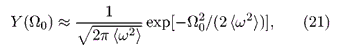
In the case of strong phase fluctuations, the frequency spectrum has the Gaussian shape independently of the choice of the spatial spectrum Φ(κ). The power spectrum of the interferometer signal is described by the relation
where
Here, J0(κρx) and J2(κρx) are the Bessel functions of the zero order and second order, respectively, Z is the thickness of the layer of inhomogeneities, ω0 is the frequency of reception, ωp is the electron plasma frequency, c is the speed of light, N is the unperturbed component of the electron number density, and V^ and ρ^ are the projections of the interferometer baseline and the solar-wind velocity on the plane perpendicular to the direction of the radiation propagation. The transverse projection of the baseline is aligned with the X axis, i.e., ρ^ = (ρx, 0).
In Eq. (21), √<ω2> is the half-width of the spectral line. The quantity <ω2> is the variance of the interference-frequency fluctuations [21] and is proportional to the intensity of electron-density fluctuations. The spectrum half-width linearly depends on the velocity absolute value. The dependence of the spectrum half-width on the mutual orientation of the interferometer baseline and the transfer velocity of the inhomogeneities is determined by the factor
where α0 is the angle between the velocity vector V^ and the x axis along which the baseline vector ρ^ is oriented. The spectrum half-width is maximum for the baseline orientation along the drift velocity of inhomogeneities and minimum in the case of mutually perpendicular directions of ρ^ and V^.
In the case of strong phase fluctuations, the spectrum width depends on the combination of the parameters of the turbulent medium and is determined by the strength of its influence. Consequently, one can qualitatively estimate the medium state by the relative broadening of spectra of the sources located at different angular distances from the Sun and measured simultaneously at several bases.
4.2. Results of experiments
When processing the experimental data of VLBI observations, the power spectrum of the interferometer signal was calculated. The propagation medium was diagnosed under the assumption that the main contribution to strong perturbations of the signal phase upon radiation propagation in a turbulent medium is given by large-scale inhomogeneities, whereas small-scale ones form the weak background of phase fluc-tuations of the transmitted radiation [26]. In this case, the power spectrum is of Gaussian shape at the background of a decreasing power-law function. On the basis of these assumptions, we analyzed the intensity of strong large-scale inhomogeneities by the spectrum width. Study of the shape of the "wings" of the power spectrum of the interferometer signal allowed us to draw some conclusions on the distribution of small-scale inhomogeneities.
In Table 3, a list of the sources observed in the INTAS00.3 experiment in December 1, 2000, the angular distances from the sources to the Sun for the moment of observation, and the used interferometer baselines are presented.
TABLE 3. Sources and used interferometer baselines in the INTAS00.32 experiment.
Source
θ, deg
Baseline (the projection length, km)
1555-140
8.6
Medvezhji Ozera - Hartebeesthoek (7860)
1524-136
14.2
Medvezhji Ozera - Noto (2 706)
1514-241
14.2
Medvezhji Ozera - Hartebeesthoek (6825)
Medvezhji Ozera - Noto (2 520)
Hartebeesthoek - Noto (5 523)
1504-167
17.3
Medvezhji Ozera - Hartebeesthoek (7589)
Medvezhji Ozera - Noto (2 660)
Hartebeesthoek - Noto (5 937)
1741-038
27.2
Hartebeesthoek - Noto (6 496)
3C279
51.0
Medvezhji Ozera - Hartebeesthoek (8026)
Medvezhji Ozera - Noto (2 679)
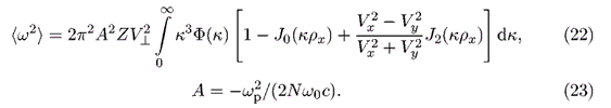
The influence of the interplanetary plasma on the instrument signal is illustrated in Fig. 9 showing the dependence of the half-width Δf of the power spectrum on the angular distance θ between the radio source and the Sun. We adopted the half-width of the Gaussian function approximating the experimental spectrum as the spectrum half-width. The vertical bars in Fig. 9 denote deviations of the experimental spectrum from its approximation. The power spectra have the largest width for the sounding paths close to the Sun, at which the influence of the turbulent medium on the propagating radiation is large. The spectrum of a signal from the source whose radiation propagates through the region not influenced by the solar-wind plasma (at θ = 51°) is a narrow spectral line. For θ < 5°, where the perturbations are most intense, the signal coherence is totally broken.
Fig. 9
The considered method of studying a turbulent medium is most informative for weak phase fluctuations, since it allows one to obtain the index of spatial spectrum of the inhomogeneities and the solar-wind velocity. To illustrate this specific case, we selected the correlation-signal samples obtained for relatively weak phase perturbations. This condition was satisfied for the observation data of the sources located at angular distances θ > 10° from the Sun. Each sample was subject to the spectral processing, before which an additional phase shift of Θ = π/2 was introduced in it.
The value of p was estimated as follows: a power-law function coinciding with the envelope of spectral "wings" was plotted on the experimental spectra in the logarithmic scale. The relationship between the envelope and the index p of the spatial spectrum was found according to Eq. (16). Beforehand, the boundary frequency F0 and the frequency FT of spectrum kink (18) were estimated. For that, the solar-wind velocity in the studied region R > 40RΟ was assumed equal to V^ = 450 km/s, and the outer turbulence scale Λ0 = 106 km. A part of the spectrum at the frequency interval F > Δf, where Δf is the spectrum half-width, was studied if the signal power exceeded the noise three times.
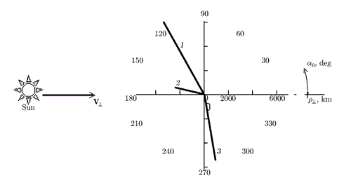
Below, we consider the sample experimental power spectra plotted by the results of observations of the source 1514-241 located at the angular distance θ ≈ 14° from the Sun. The projections of the used baselines onto the image plane of the 1514-241 source are shown in Fig. 10. The radius in the polar coordinates correspond to the length ρ^ of the baseline projection, and α0 is the angle between the projections of the baseline ρ^ and the solar-wind velocity V^ onto the plane perpendicular to the direction of radiation. It was assumed that V^ is directed from the Sun to the source. The digits 1, 2, and 3 in Fig. 10 denote the following baseline projections: Medvezhji Ozera - Hartebeesthoek, Medvezhji Ozera - Noto, and Hartebeesthoek - Noto, respectively.
Fig. 10
Fig. 11, 12
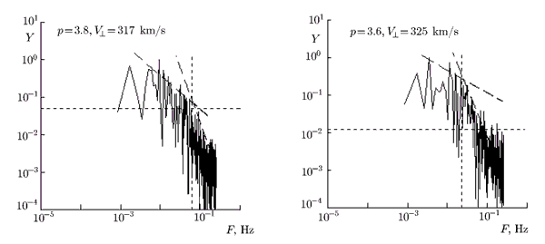
The power spectrum Y(F) of the interferometer signal, plotted in Fig. 11, was calculated by the results of observations using the Medvezhji Ozera - Noto interferometer. The transverse projection of the interferometer baseline was oriented at an angle α0 ≈ 12° to the direction from the Sun to the source, and the length of the baseline projection at the initial moment of the observation session was ρ^ = 2518 km. In Fig. 11, the spectral kink is clearly seen, by the frequency FT of which the solar-wind velocity at the sounding path was estimated according to Eq. (18) as V^ = 2FTρ^ = 317 ± 10 km/s. The horizontal dashed line denotes the level of noise power below which the spectrum was not analyzed. The frequency FT corresponds to the intersection of the functions Y2 = F -p+3 and Y2 = F -p+l (see Eq. (16)) approximating the spectrum at the two frequency intervals, i.e., F < V^/(2ρ^) and F > V^/(2ρ^). The index p of the spatial spectrum, estimated by the spectral index of these curves, equals 3.8.
The considered method assumes that the spectra obtained from observations using the interferometers with baselines oriented mainly along the transfer velocity of inhomogeneities should contain oscillations determined by the ratio of the velocity projection to the length of longitudinal baseline component. In the given spectrum, the oscillations are not seen. The preliminary calculation using Eq. (13) showed that for α0 = 12°, the fluctuations are weak (see Fig. 7). Moreover, the velocity fluctuations in the studied region could be significant, which would result in smoothing the spectral minima. High noise level in the range F > V^/(2ρ^) made it impossible to estimate the transfer velocity of inhomogeneities by the location of local spectral extrema.
Figure 12 shows the spectrum plotted by the data of the same observation session at the Medvezhji Ozera - Hartebeesthoek baseline. The index p of spatial spectrum, estimated by the experimental power spectrum, equals 3.6. During the observation session, the angle between the baseline and the direction from the Sun to the source was α0 ≈ 60°, and the length of the baseline projection was 6825 km. Using the spectrum-kink frequency FT = V^/(2ρ^), the transfer velocity of inhomogeneities was obtained: V^ = 325 ± 14 km/s.
Fig. 13, 14
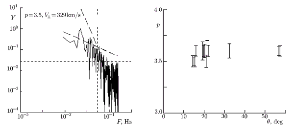
The spectrum built by the measurements at the Noto - Hartebeesthoek baseline, located at the angle α0 ≈ 81° to the velocity direction, is shown in Fig. 13. In this case, the spectrum kink is very weakly pronounced. Therefore, the error of the obtained solar-wind velocity is large: V^ = 329 ± 40 km/s. The estimate of the spatial-spectrum index obtained using the frequency range F < V^/(2ρ^) is p = 3.5.
The observations of six sources allows us to obtain the mean solar-wind velocity V^ = 342 ± 17 km/s.
Figure 14 shows the p values measured for different angular distances from the Sun. The dependences of the spectral index and the solar-wind velocity on the angular distance from the Sun and the baselines orientation were not revealed when processing the experimental data. This result could be expected, since we study the range of heliocentric distances with the established solar-wind plasma flow [9], for which the drift velocity of inhomogeneities and the spectral index do not vary significantly.
From processing the observation results for six sources in the INTAS00.3 experiment, the mean value p = 3.57 ± 0.06 of the spectral index was obtained. This value is close to the Kolmogorov-spectrum index (pk = 11/3) and agrees with the experimental results of the solar-wind studies employing different methods [9, 21].
The described method allowed us for the first time to estimate the drift velocity of inhomogeneities and the spatial-spectrum index of electron-density fluctuations independently from each other, unlike the earlier interferometric experiments on radio-raying the solar wind. Usually these parameters are mutually dependent, i.e., one of them is assumed known when estimating the other one. Using the method of weak amplitude scintillations, one usually obtains the drift velocity and the spectral index of electron number density for inhomogeneities with scales from tens to hundreds km [9], whereas in our case, estimates of the medium parameters are made for scales comparable to the projections of baselines of the radio interferometric complex, i.e., plasma inhomogeneities with sizes from hundreds to thousands km are studied. The obtained values of spectral index and the velocity allows us to confirm the applicability of the frozen-in hypothesis and the Kolmogorov spectrum for description of spatio-temporal measurements in the solar wind at large distances from the Sun (R > 40RΟ) in the range of turbulence scales which was almost not studied earlier.
Despite of the large number of observation sessions (2-3 scans of each of the six sources for measurements using 2-3 baselines), the number of samples satisfying the necessary conditions (the smallness of phase-difference fluctuations and the wide spectral width) was not enough for a statistical analysis. For interpreting the data (i.e., for obtaining the spatial-spectrum index and the transfer velocity of inhomogeneities) the spectrum must be built in the frequency range including its specific features such as the kink point and oscillations, which are located at frequencies F > FT = V^/(2ρ^). In the described experiment, the data correlation was carried out with a too long integration time of 2 s, which in most cases did not allow us to obtain the spectra in sufficiently wide frequency band for comprehensive analysis. For this reason, the high-frequency part of the spectrum, which is of interest to us, could not be studied.
Consider the results of spectral data processing obtained for strong phase fluctuations of the received radiation.
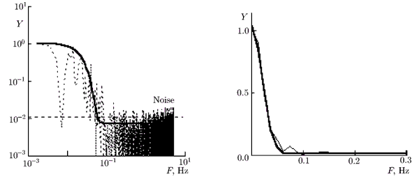
Within the framework of the INTAS99.4 experiment in December 2, 1999, VLBI observations of a group of 6 sources located at angular distances of 2° to 25° from the Sun were carried out. Each of the sources was scanned three times, the duration of each scanning session was 10-15 min, and the interval between the sessions was 1 h. The observations were performed under conditions of enhanced solar-flare activity, which, along with the close location of the sounding path to the Sun, resulted in attenuation of the signals of most observed objects due to the influence of intense solar-wind inhomogeneities and made it difficult to estimate the medium parameters. A sufficiently strong interference signal, clearly discernible at the noise background was obtained only for the NRAO 530 source which was located at the angular distance θ ≈ 17° from the Sun during the observations. The radiation flux of this source at a frequency of 1665 MHz was 5.6 Jy, whereas the radiation flux of the other five sources did not exceed 0.5 Jy.
For analysis of the results of observations of the NRAO 530 source, we selected the measurement data obtained for weak amplitude and strong phase fluctuations. The correlation was performed after preliminary averaging with the integration time τu = 0.1 s, which allowed us to study the spectrum in the bandwidth δf = 5 Hz. Spectral processing of 14 samples obtained at 7 baselines of the radio interferometric complex was performed. Additional cleaning of the signal from spurious noise was performed using the following well-known scheme [27]. A discrete sample of the correlation signal was split into equal intervals, fast Fourier transform and its complex conjugate were calculated for each interval, and then averaging over all the intervals was performed.
Fig. 15, 16
A sample power spectrum of the interferometer signal measured at the Noto - Svetloe baseline is shown in Fig. 15 on the logarithmic scale (dashed line). According to the findings of the theoretical analysis, the power spectrum for strong fluctuations of the received radiation is described by the Gaussian function whose half-width equals the variance of the interference-frequency fluctuations [22, 23]. The Gaussian function approximating the spectrum is plotted by a solid line in Fig. 15. The horizontal dashed line marks the noise level. The averaged spectrum is shown by a thin line in Fig. 16, the approximating Gaussian function is plotted by a bold line.
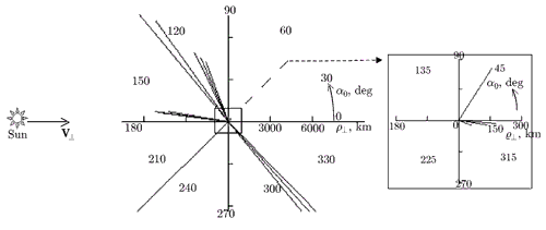
Figure 17 shows the baseline projections onto the image plane of the NRAO 530 source, where α0 is the angle between the baseline projection and the radial direction from the Sun to the source. Table 4 presents the used baselines, the lengths of their transverse projections, and the angle α0 values.
Fig. 17
TABLE 4. Interferometer baselines used in the INTAS99.4 experiment.
Baseline
α0, deg
Length of baseline projection, km
Medvezhji Ozera - Svetloe
57.7
280
Medvezhji Ozera - Hartebeesthoek
-45.8
7842
-48.1
7643
-50.9
7485
Medvezhji Ozera - Pushchino
-4.9
89
-23.2
54
Medvezhji Ozera - Shanghai
-135.6
6402
Hartebeesthoek - Noto
116.6
6096
113.9
6136
111.4
6209
Hartebeesthoek - Svetloe
130.0
7720
125.9
7569
Noto - Svetloe
172.6
2698
170.9
2203
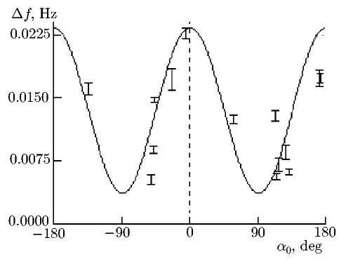
We analyzed the dependence of the half-width Δf of the interferometer-signal spectrum on the angle between the transverse projections of the transfer velocity of inhomogeneities and the interferometer baseline.
Fig. 18
To estimate the value of Δf, each spectrum was approximated by a Gaussian function whose half-width was assumed equal to the half-width of experimental spectrum. In Fig. 18, the vertical bars show the mean Δf values calculated for each sample. The bar length corresponds to the mismatch between the initial curve and its approximation. The abscissa axis corresponds to the angle between the baseline projection and the Sun-source direction, along which, as was assumed for calculations, the solar-wind velocity was oriented. The solid line shows the theoretical curve plotted according to Eq. (22). As follows from the plot, the experimental data are in good agreement with the model calculations.
Thus, the data of VLBI experiments on studies of solar-wind plasma show satisfactory agreement with the results of theoretical analysis as related to the calculation of the index of spatial spectrum of electron-density fluctuations and solar-wind velocity for weak phase fluctuations of the received radiation. However, the statistical analysis of the measured parameters cannot be considered complete, since the observations for quiet solar conditions were insufficient for revealing their dependence on the angular distance from the Sun and the baseline orientation.
To obtain reliable data on solar-wind plasma in one measurement cycle, it is necessary to observe as many radio sources as possible. The interval of angular distances of the radio sources from the Sun should be chosen sufficiently wide, i.e., from small angles (θ ≈ 2°-3°), at which the solar-wind formation occurs, to large angles (θ ≈ 60°-80°), at which the disturbances introduced by the near-solar plasma are small compared with the influence of the interplanetary plasma. One should take into account that the influence of the medium on the interferometer signal is significant in the region close to the Sun (2 ° < θ < 8°); hence, the radio sources with radiation fluxes exceeding 3 Jy should be chosen for studying the plasma in this region. To minimize the influence of the Earth's ionosphere to the measurements, the position angle of each antenna observing a source must exceed 15°.
The correlation analysis must be performed with small integration time (depending on the studied region and the length of the used baselines), which allows one to study the power spectrum of the interferometer signal in a sufficiently wide frequency range including the spectrum features such as the frequencies of the main maximum, the spectrum kink, and the local maxima. In addition, the duration of observation sessions for each source should be about 10-15 min to achieve a high frequency resolution.
5. CONCLUSIONS
In this paper, we generalize the experience of using the Canadian recording system S2 in Russia within the framework of the Low-Frequency VLBI-Network (LFVN) project. The S2 system demonstrated very good parameters, reliability, robustness, and extreme flexibility for use, which is especially important in Russia where the radio telescopes are equipped poorly and with heterogeneous apparata. The period of using the S2 system (from 1993 to 2000) was probably the most productive in the history of national astrophysical very-long baseline radio interferometry. Several Russian telescopes simultaneously took full part in international experiments, including those on ground-space radio interferometry (the VSOP project). In the observations whose program was formed by the applications of Russian scientists new results on OH masers, quasars, and solar wind were obtained. Since the S2 system is still the most popular VLBI recording system in Russia and operating at many international radio telescopes, it seems expedient to try reviving regular observations with the use of the S2 system by reaching a cooperation agreement with the Australian or Japanese correlators.
We discussed the main results of two most interesting LFVN observation sessions in 1999 (INTAS99.4) and 2000 (INTAS00.3), carried out at a wavelength of 18 cm and processed by the Canadian correlator in Pentictone. The LFVN images of the 1418+546 and CTA 102 radio sources are presented and analyzed, and some results on the sources 0420-014, 0420+022, 1308+326, 1345+125, and 1803+784, which were not included in [8], are presented. For all objects except the 1345+125 source, the quality of uv-plane filing achieved by observations at 6 antennas can be considered satisfactory, since small, medium, and long baselines were realized during the experiment. Nevertheless, it is extremely important to increase the number of participating nodes of the VLBI network for increasing the dynamic range of the maps and improving their reliability. For example, increasing the number of antennas from six to seven leads to a significant (by 40%) increase in the number of possible baseline projections.
The methodology of VLBI studies of solar-wind plasma using the method of radio-raying by radiation of natural sources was presented in detail and theoretically justified. The basic software for spectral processing of the interferometer signals distorted by the influence of a disturbed medium was created and debugged. Theoretical analysis and numerical modeling showed that one can study large-scale inhomogeneities in the solar corona or supercorona by the spectrum of the interference response using multi-element VLBI complexes for observations of radio sources in wide ranges of elongation and position angles with respect to the Sun. Processing of the experimental data allowed us to estimate the index of spatial spectrum of electron-density fluctuations and the drift velocity of inhomogeneities in the sounded region. For the first time the solar-wind velocity and the spectral index were obtained independently for inhomogeneity scales comparable with the baseline lengths, i.e., from 2000 to 9000 km. These parameters allow us to confirm the applicability of the frozen-in hypothesis and the Kolmogorov spectrum for describing the spatio-temporal measurements in the solar wind at large distances from the Sun (R > 40RΟ). We plan to continue the observations with account of the recommendations developed in the course of data processing.
REFERENCES
I. Molotov, S.Likhachev, A. Chuprikov, et al., Proc. IAU Symposium 199, 30 November~4 December 1999, Pune, India (1999), p. 492.
V. A. Alexeev, V. I.Altunin, Yu. N. Gorshenkov, et al., Proc. Conf. on Modern Problems and Methods of Astrometry and Geodyn., Sept. 23-27, 1996, St. Petersburg (1996), p. 156.
W.H.Cannon, D.Baer, G. Feil, et al., Vistas Astronomy, 41, 297 (1997).