Fifth European Conference on Space Debris
30 March - 2 April 2009
ESA/ESOC
Darmstadt, Germany
Analysis of Object Observations using a 1.8-Meter Telescope
Paul Kervin, Paul Sydney, Mark Bolden, Tom Kelecy
AMOS Detachment US Air Force Research Laboratory Maui, Hawaii, USA
5th European Conference of Space Debris,
March 30 - April 2 2009
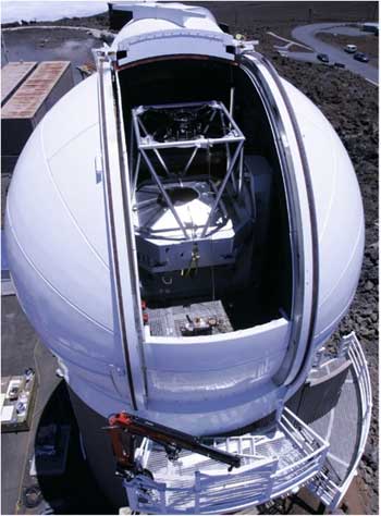
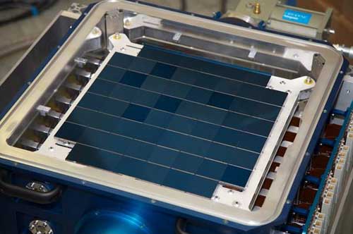
Pan-STARRS
- Panoramic Survey Telescope And Rapid Response System
- Designed for astronomical mission
- Prototype system can be used for satellite observations
- Specifications
- 7 square-degree field of view
- 1.8-meter aperture
- 1.4 gigapixel camera
- 38k x 38k array
- 0.3 arcseconds/pixel
- High-accuracy position information
- 2.8 gigabytes/image
- 2-3 terabytes of data per night
Located at 10,000-ft summit of Haleakala
Tracking mode:
- Sidereal tracking (astronomical observations)
- Tracking off (satellite observations)
- Optimized for geostationary satellites
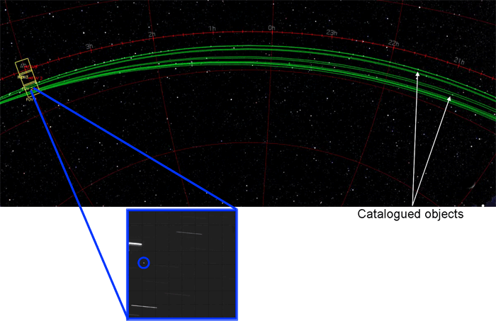
Pan-STARRS Search Strategy
- Slew to same RA/Dec fields, stop
- Stars streak
- Same stars in each Dec field
- Geostationary objects appear as points
- Optimized for geostationary objects
- Greatest sensitivity to geostationary objects
- Lesser sensitivity to all other objects
.95 < n < 1.05
e < 0.1
i < 5.5
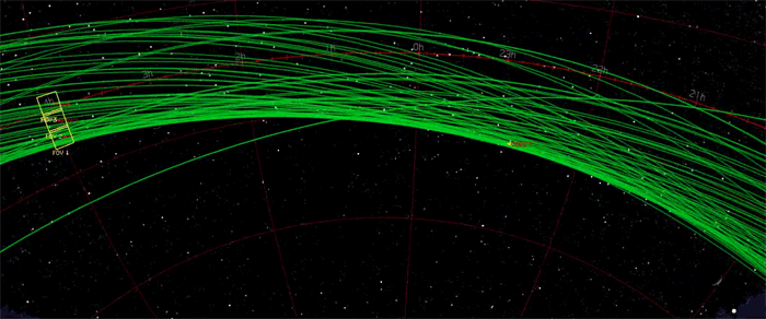
Pan-STARRS Search as implemented for Dec 2008
- Optimized for geostationary objects
- Greatest sensitivity to geostationary objects
- Lesser sensitivity to all other objects
- Trade-offs
- RA selection, integration time, fence height, overlap, filter selection
.9 < n < 1.1
e < 0.1
i
Optical Search
- “Fence” is not leak-proof
- Only 3 declination fields high (~8 degrees)
- Can lose objects above or below that fence
- Weather can put leaks in the fence
- Fence is optimized for geo orbits
- But…
- Multiple observations of each satellite over 10 minute period
- Less than 1% of geo satellite orbit
- Astrometric accuracy good in center of FOV, some distortion errors near edge (2-6 arcsecs)
- Will improve over time with goal of 0.25 across FOV
- Can usually get a reasonable satellite fingerprint
Pan-STARRS Data Reduction
- Several terabytes per night
- Reduction has to be automated
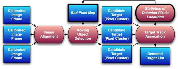
- Steps include
- Data transfer
- Pixel Non-Uniformity Correction (PNUC)
- Star matching
- Image registration
- Background/clutter rejection (including cosmics)
- Frame-to-frame association of objects
- Challenges
- False alarms
- Nonlinearity of pixel response
- Loss of effective area on focal plane
- Cosmic rays
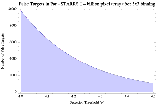
Data Reduction Challenges
Pixel detection, P is based on combining a stack of N image frames in Constant False Alarm Rate (CFAR) Detection with threshold, T as:
Pmax – Pavg(w/o max) > T • σP(w/o max)
Problem: Statistics from a large number of pixels still results in ~2600 false alarms for detection threshold, T of 4.3σ for each frame
Approach: Require 2 or more adjacent pixels for a valid detection
- Does reduce detection sensitivity to some degree
- In general, spot size > IFOV assures valid target covers 2 or more pixels
Problem: PNUC does not address pixel response non-linearity, i.e. “warm pixels” which can create false targets
Approach: Perform detection step twice.
- First, analyze detections over many observations and identify pixels producing frequent detections. Targets are moving with respect to FOV.
- Create a mask image ignoring these high detection rate pixels
- Repeat detection step using mask image. For PS1, generally <0.1% of pixels are masked
Future: Calibration screen with “leaky fibers” fed by a monochromator will calibrate pixel response linearity
Problem: 0.143 m 2 PS1 array with 75µm CCD thickness results in 200-300 cosmic ray hits per exposure with an average length of 3-4 pixels
- Track association reduces some of the false targets
Approach: Implementing Dokkum Laplacian Edge Detection Algorithm for detecting CRs
- By implementing the algorithm at the detection step, the processing requirements can be greatly reduced
- Use of simple shape parameters or PSF matching has had limited success
Problem: Bad and hot pixels along with gaps between the chips in the sensor mosaic result in a 7-11% loss in detection area
- M out of N detections allows for some missing detections
Approach: When detections are paired to form the endpoints of a potential track, intermediate detection points are counted if they fall in a detection loss area.
- PS1 Rule of Thumb: 3 detections predicted in loss areas are considered a single valid detection.
Detection Sensitivity
- Performance based on 2 Dec 2008 observations
- 3x3 pixel binning
- Observed in Sloan Digital Sky Survey (SDSS) “w” filter
- 5 second exposure time
- Airmass ranged from 1.15 to 2
- Binned IFOV: 0.75 arcsecs
- Spot size (FWHM): 0.85 arcsecs
- Sensor gain: ~1 e- / DN
- Sensor noise: < 8 e-
- Sky background: 350 – 550 e- (20.5 – 21 Mv / arcsec2)
- Total measured RMS noise (σ): 20 – 24 e- (varies with airmass)
- Detection threshold: 4.3σ
- Minimum detection size: 3 pixels
- Estimated detection limit is ~21.5 mags in SDSS w filter
�- Faintest target detected for Dec 2008: 21.0 mags
Pan-STARRS Data Analysis
- Input data
- Accurate metrics
- Multiple observations over a 10 minute period
- <1% of GEO orbit
- Analysis method
- Use Gauss’ method to determine orbit using 3 of the observations
- Use Least Squares method to refine that initial orbit using all observations
- Some orbital elements are more accurate than others
- RAAN and Inclination (orbit orientation) fairly well determined
- Mean motion and Eccentricity require more data
- Can get a satellite fingerprint
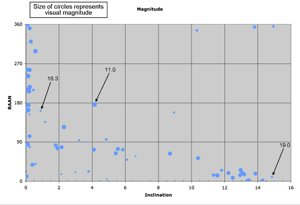
- Brightness (average and variation)
- Inclination
- Right Ascension of Ascending Node
- These parameters are usually slowly varying
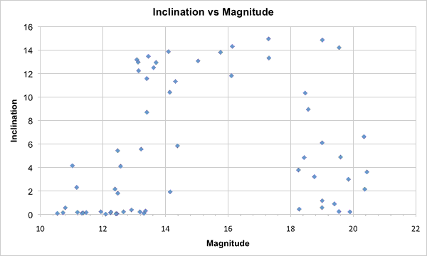
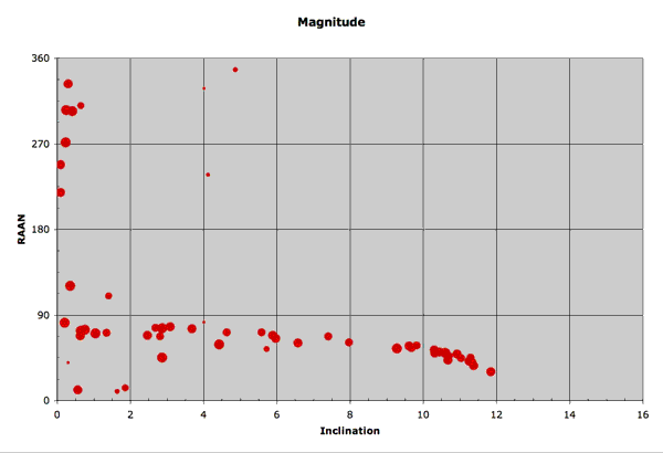
Fingerprints
Fingerprints: most useful if they are widely distributed
August 2008 Data
- Clustering: low inclination and bright
- Most likely cataloged objects
- Objects we most want to fingerprint are spread nicely
August 2008 Data
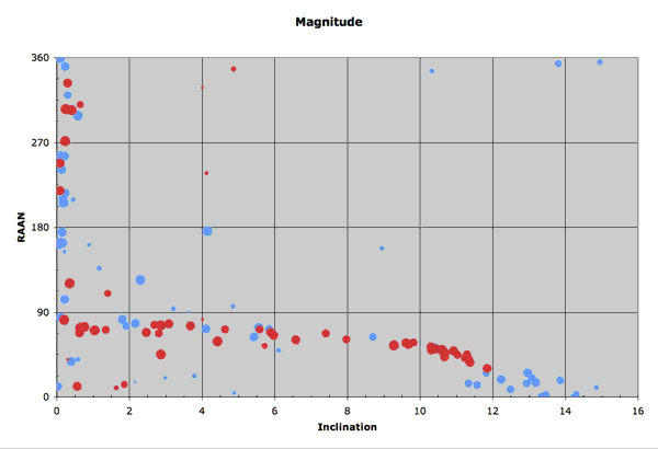
December 2008 Data
August and December 2008 Data
Fingerprint Observations
Possible causes for differences in “fingerprints” between the two datasets
- December data was less noisy (better alignment, focus, etc.)
- Long time period between observations
- Possibly different satellite populations
- Uncertainties in the values of the parameters
- Values can change over several months due to environmental orbit perturbations
Magnitude, Inclination, RAAN are useful parameters
- Nice spread in satellites in this parameter space
- The parameters are, for the most part, slowly changing
- Should be very useful in linking night-to-night observations
Concluding Remarks
- Care should be taken in interpreting this data
- Don’t have the luxury (so far) of years of observations of the satellite environment
- Very small sample, so statistics are poor
- Should be cautious about inferring population distributions
- Sensitivity will increase as system is optimized
- Alignment and focus
- Utilize unique aspects of Orthogonal Transfer CCDs
- Should be able to link many observations from one night to another using satellite fingerprints
Размещено 17 апреля 2009
Все представленные материалы размещены с согласия авторов докладов
|