The previous tables are now illustrated by seven graphs. They give a global view of the situation in the geostationary orbit and the distribution of the objects in each category.
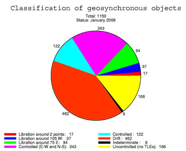
Figure 7: Number of objects in each category
Please note, that the 122 controlled objects consist of the 75 objects in class C2 (only East-West station keeping) and the 47 objects in Section 4.1 where no TLEs are available.
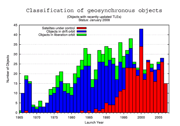
Figure 8: Number of objects in each category according to the launch year.
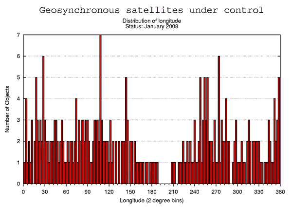
Figure 9: Distribution of the longitude of the 318 satellites under control (with updated TLEs).
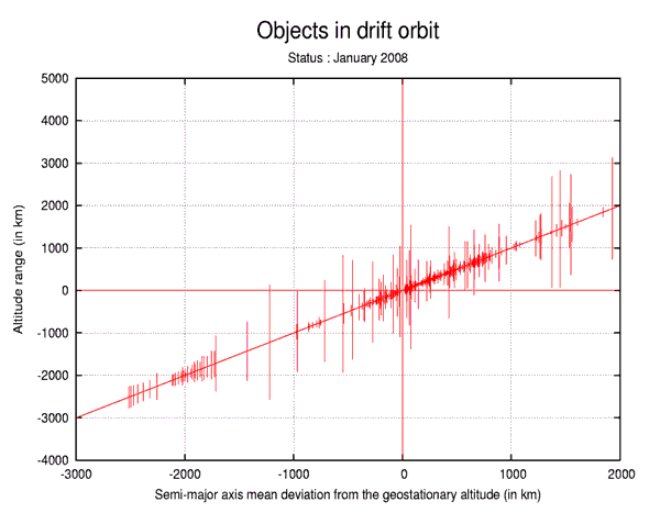
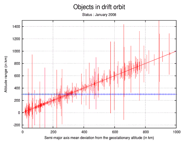
Figure 11: Distribution and altitude range of the objects in drift orbit.
This figure illustrates the distribution of the objects in drift orbit. Each vertical line represents one object.
The horizontal axis gives the semi-major axis mean deviation from the geostationary altitude, which is inversely proportional to the mean drift rate of the object.
The vertical axis gives the perigee and apogee mean deviation from the geostationary altitude. The altitude of the object librates between these two values. One can see that if the eccentricity is large, the object can go through the geostationary altitude.
Figure 11: Zoom in the distribution and altitude range of the objects in drift orbit.
This figure is a zoom of the previous figure. This area is important because, according to the IADC recommendations, a satellite should be reorbited at its end-of-life to a graveyard orbit with a perigee altitude which is about 300 km above the GEO ring.
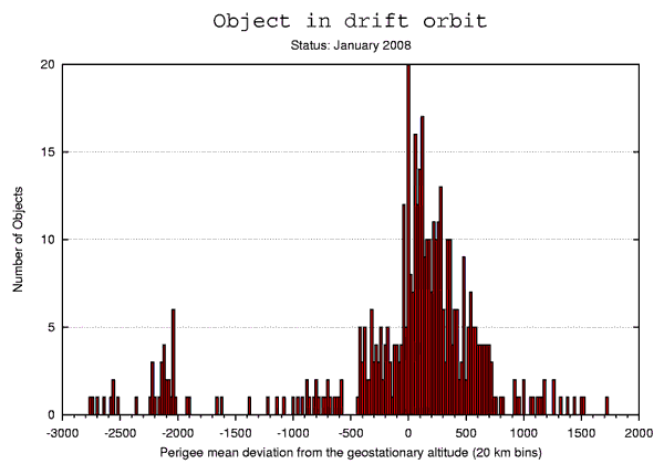
Figure 12: Distribution of the perigee mean deviation from the geostationary altitude.
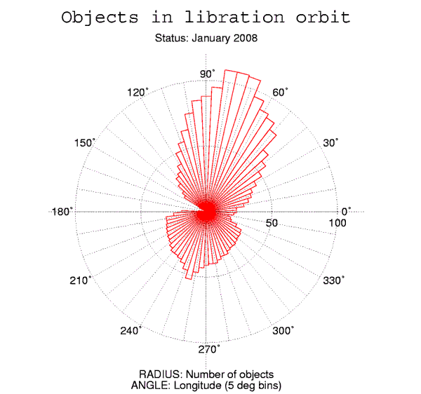
Figure 13: Distribution of the objects in libration orbit in 5-deg bins of geographic longitude (objects with updated TLEs only).
This figure illustrates the distribution of the objects in a libration orbit. For every interval of 5 degrees, the number of objects librating through this longitude interval is given. For instance, an object librating between 64 deg E and 86 deg E is counted in the 5 intervals 62.5-67.5, 67.5-72.5, 72.5-77.5, 77.5-82.5 and 82.5-87.5.
For the same reason, all the objects classified as librating around the Eastern stable point or around the 2 stable points are counted in the interval 72.5-77.5, because they all go through the longitude 75 deg E. Thus, the number of objects at 75 deg E shown in this figure is equal to the sum of the objects in the L1 and L3 categories.
|