ON A NEW THEORY OF THE GEOSTATIONARY SATELLITE MOTION AND ITS APPLICATIONS

R. I. Kiladze

Abastumani Astrophysical Observatory, Georgia (FSU)

Launching artificial Earth satellites into the geostationary orbits (GO) began about 40 years ago. At the present time the geostationary satellites (GS) moving in a sharp resonance with the Earth rotation have the most wide applications in resolving many practical problems, mainly those related to the TV-communications, intercontinental communication and military purposes.

After expiration of its active period a GS becomes a passive object and is transferred onto a higher or lower orbit in the neighbourhood of the GO. According to the statistics by January 2005 there were 346 GS working in the GO and their total number was 1124.

Besides of observable objects there are ten thousand small fragments, smaller than 1 m in size, which are small space debris (SD) moving in the vicinity of the GO. They are accompanying every launch of the GS and are created as a result of the GS explosions.

According to the recent investigations the number of such explosions is 12; 2 of them were the Russian GS (Ekran 2 and Ekran 4) and 10 were the U.S. “Transtages”. Maybe this number is underestimated; therefore, in addition to elaboration of reliable methods for the detection of explosions by direct observations, it is necessary to dispose of the program for the search of all lost objects, and especially, of potentially dangerous ones for working GS.

These fragments are endangering the existence of the GS because of the possibility of collisions. The number of small fragments is growing with time (their existence time-span in the region of the GO is unlimited) and the probability of their collision with the SD grows. Recent investigations of the evolution of 456 uncontrolled GS observed more than 1000 sharp changes in their drift, which may be explained in terms of collisions with small SD [1].

The main problem of the GS motion control is still related to the cataloguing of all observed small objects moving in the GO region.

For elaborating a model of choking up the GO region by the SD it is necessary to have a reliable theory of the GS motion by which the available observations and orbital elements might be represented on the long time-span. It is also necessary to compile the software for calculation of the orbital evolution for hundreds of fragments in a short time.

Our task was to construct a simple method to calculate the long-period evolution of the real GS orbits. The elaborated method, based on observations made on the time-span of 1000 through 2000 days with the mean square error σ in the range of 0°.025 through 0°.045, allows to represent the orbital evolution on the time-span of 7000 through 10000 days with an error of 0°.1 – 0°.2.

The theory has been tested by means of representation of long series of Two-Line Orbital Elements (TLE) of the NASA Goddard Space Flight Center and of the osculating elements (OE) determined by us directly from astrometric observations [2].

The principal peculiarity of the motion of a GS is the exact 1:1 commensurability of its mean daily orbital motion n with the Earth’s rotation velocity S₁. In the case of absence of perturbations due to the nonsphericity of the Earth’s shape and to the luni-solar attraction, the GS once launched at some geographical longitude would always rest there. However, under the influence of ellipticity of the Earth’s equator, it begins to move like a pendulum near two stable points of libration with longitudes 75°Е and 255°Е. Because of the asymmetry of Earth’s equator the periods of the small oscillations around these points differ by 110 days, being equal to 840 and 950 days, respectively.

To simplify the representation of such a motion Gedeon [3] has introduced a special system of coordinates, called by him stroboscopic.

In this system instead of the continuous time the discrete time-time-moments are used as the argument of the equations of motion separated by daily intervals, and the phase plane of the stroboscopic longitude λ and drift dλ/dt is introduced in terms of orbital elements as follows:

          

where M is the mean anomaly, Ω is the longitude of the ascending node, ω is the argument of the perigee, S is the Greenwich sidereal time, Ω₁ and ω₁ are secular changes of the node and perigee longitudes.

In the stroboscopic system of coordinates, – in the case of an exact commensurability of motions, – the central body and a satellite seem to be motionless, and in the case of an inexact commensurability the satellite would seem to slowly move along a trajectory. Such a picture may be observed if the system, “the Earth – a satellite”, is in the darkness, being periodically illuminated by short light-flashes.

The stroboscopic system has properties of the inertial and noninertial (rotating) coordinate systems. Introduction of this system essentially simplifies the equations describing the long-period motion of the GS, but results in a loss of the short-period oscillations.

To describe the GS motion A. Sochilina in 1985 has used the Laplace plane [4], being first applied by H. Struve [5] to the satellite motion. It passes through the vernal equinox and is inclined by some angle Λ (depending on the semi-major axis of an orbit) to the geoequator. For the GS the angle Λ is equal to 7°.34188.

The physical meaning of the Laplace plane is the following. Due to the equatorial bulge of the Earth a couple of forces are created which are trying to make the plane of the GS orbit to coincide with that of the geoequator; as a result the plane of the orbit (in the case of absence of other forces) precesses, being constantly inclined to the geoequator. On the other hand the common attractions of the Moon and the Sun try to make this plane to coincide with the ecliptic.

The resultant of these two couples of forces compels the GS orbit plane to precess by the constant inclination to a plane lying between the geoequator and the ecliptic and called the Laplace’s plane.

The choice of the Laplace plane gives some advantages over other planes of reference: relative to it the inclination of orbit i changes (because of inclination of lunar orbit to ecliptic) only in limits of ±0°.5 and the longitude of the node Ω and the perigee argument ω become practically linear functions of time. The resonance equation for the stroboscopic longitude λ also becomes simpler.

As a result the problem may be resolved by use of the first order theory with small corrections for the second order only.

Usually the precision of some osculating orbital elements is not satisfactory, – especially for the calculation of satellite’s drift dλ/dt – but the derivatives of λ with respect to time may be improved by use of the data of preliminary orbits combined with the long-period motion theory.

In the process of work with the Catalog of improved orbital elements [6] in 1996 it was pointed out that on the 1000-day span some GS show considerable systematic differences in the longitude (in some cases reaching several degrees) between observed “O” and calculated “C” values.

After estimation of the theory accuracy R. Kiladze [7] assumed that these discrepancies could result from accidental changes in dλ/dt which in their turn are caused by the collisions with small particles.

Perturbations of the GS orbital elements may be found from the Lagrange equations. The perturbing function due to the geopotential U, the luni-solar perturbations R_L, R_S and the radiation pressure R may be expressed in terms of orbital elements referred to the Laplace plane [8]:

          (1)

where GE is the gravitational constant, a_e , the mean equatorial radius of the Earth, G_lm = C_lm √-1 S_lm, C_lm, S_lm, the geopotential parameters, E_lmk(Λ), D_lkp(i), the inclination functions and X_l-2p+q^-l-1,l-2p(e) , the Hansen coefficients calculated in [9], M, Ω, ω, e, i, a, the GS orbital elements.

The perturbing function due to the Moon is expressed as follows:

          (2)

where       ε is the inclination of the ecliptic to the geoequator, Ω_L, ω_L, e_L, i_L, a_L, the orbital elements of the Moon.

One can obtain the perturbing function due to the Sun by changing the index L in (2) to the index S.

According to Kepler’s third law

          

The mean radiation pressure function is as follows:

          (3)

where λ_S is longitude of the Sun, the ratio of the surface area to the mass expressed in cm²/gr).

The equation for calculation of Λ may be obtained from the condition that the sum of terms of perturbing functions U, R_L, R_S, with argument Ω, be equal to zero:

          (4)

where are the mean motions of a satellite, the Moon and the Sun, respectively, expressed in radians per day:

          

At last, all resonance perturbations are accounted for by the differential equation for λ [2]:

          (5)

where A_lmkpq is the function of a, e, i and of the geopotential parameters, λ_lmkpq, the phase angle depending on λ_lm, and the geopotential parameters C_lm = J_lmcosmλ_lm, S_lm = J_lmsinmλ_lm, LSP meaning the luni-solar perturbations.

The solution of this equation is described in [10].

For simplification sake let us write the equation (5) as follows:

          (6)

where

          (7)

Choosing the Laplace plane as the basic one for the coordinate system guarantees that the change of coefficients А_i, m_i, φⁱ and s_i in (6) with time is very slow (i.e. that they are almost constant).

If these coefficients and the longitude of node Ω are constants, in the case of absence of the luni-solar perturbations, the equation (6) allows for the first integral:

          (8)

where С₁ is the integration constant, being analogous to the Jacobi’s constant in the restricted problem of three bodies and in such a case the problem can be solved in terms of the quadrature:

          (9)

          (10)

The behavior of the function Π(λ) is shown on Fig.1. It is like the asymmetric double sinusoid with maximums and minimums of different heights.

Accordingly, depending on the value of parameter С₁, the GS can move in accordance with one of the three modes– the simple libration around one from the two stable points 75°E or 105°W, the compound libration (around both points), or in the mode of the circulation (the drift) around the Earth.

Fig.1. The function Π(λ).

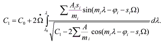
Because of the smallness of dΩ/dt, the solution of equation (6) may be expressed in the form (8), if one considers С₁, as a slowly changing function of time.

          (11)

In such a case one can obtain the derivative of С₁ with respect to time: introducing a new variable of integration dλ instead of dt by means of (8) we get:

          (12)

The exact calculation of the right-hand side of the equation (12) is not feasible since the dependence of variables C₁ and Ω on λ is unknown; but, with an accuracy acceptable for practical applications, they may be considered on short time intervals as constants equal to the average values of the quantities C₁ and Ω, respectively.

The variability of C₁ and inaccuracy of calculations by means of (10), connected with the variability of Ω with time, may be significantly diminished by introduction of the oscillating system of coordinates, attached to the Π(λ) function.

On Fig. 2 different types of motion in the phase plane are schematically shown. If the value of the drift is less then 0.3°/day, then the GS move in the mode of a libration around one of the stable points with the amplitude depending on the initial longitude.

The GS having maximum amplitudes of libration may periodically change their motion modes because of the luni-solar perturbations.

Fig 2. Different types of the GS motion in the phase plane “longitude λ vs. rate of drift dλ/dt”.

The method for calculation of the longitude just described allows to calculate ephemerides for a majority of the GS for the time intervals of several years with quite satisfactory accuracy for observers.

Further improvement of the ephemerides accuracy is possible by improving the GS orbital elements. For all this it is important to have the intermediate orbit which is maximally close to the real one.

The solution of this problem is published in [11] and [12]. Keeping the main terms in the right-hand sides, the Lagrange equations for the 4 orbital elements e, i, ω and Ω, in terms of the coordinates used, may be reduced to the form:

          (13)

          (14)

          (15)

          (16)

where

          (17)

ω, i, Ω and e denote here the orbital elements (the argument of the latitude, the inclination, the longitude of the ascending node, and the eccentricity), ω_L, Ω_L, the argument of the latitude and the longitude of the node of the Moon on the ecliptic, respectively, λ_S, the longitude of the Sun. D stands here for the light pressure, k, A, m, x^•, Ω^•_L and R^• are considered as constants.

The equation system (13-16) is actually subdivided into two systems, each containing two equations.

Multiplying equations (13) and (14) by expressions respectively, and summing them up, one can obtain the equation in complete derivatives with respect to time, allowing for the first integral:

          (18)

Using the integral (18) the solution of system (13) and (14) may be received in the form of the elliptic integral:

          (19)

In order to resolve the system (15)-(16) let us introduce new coordinates p and q by:

          (20)

and also

          (21)

where

          (22)

Then the system (15)-(16) becomes:

          (23)

The solution of the linear system (23) isn’t difficult, because the free terms in the right- hand sides of these equations are the variables found from the equation of system (18)-(19).

At last, by integrating the expression (21) the time can be calculated as the function of variable τ:

          (24)

The computer software compiled on the basis of the described solution of the problem copes successfully with the task of the orbit construction and of following its evolution on the time-span of tens of years for every known GS.

It is necessary to mark the scientific meaning of the first integral (18) obtained by integration of the Lagrange equations. After the epoch of resolving the two-body problem by Newton, in the scientific armory of celestial mechanics there appeared only a single first integral, i.e. that of Jacobi found in XIX century.

By means of the integral (18) the inclination of the GS orbit to the Laplace plane is given as the function of its longitude of the node and of the orientation parameters of the lunar orbit.

Because the oscillations of the inclination of the GS orbit are described by (18), we named this integral by the Russian word “Kren” (the tilt, the banking angle) and the constant C₂ by the Kren constant, respectively.

It is shown in [11] and [12] that in the general case the change of the value of C₂ is not greater than C₂×10^-8, i.e. C₂ is practically constant. Consequently, (18) is always highly accurate.

Today the constants C₁ and C₂ are used for the identification of unknown GS discovered in the process of the sky surveillance with objects lost in the past. But with the science progress each of the known first integrals has found a new, sometimes unexpected application. We should expect that the Kren integral will not be an exception of this rule.

As it was mentioned above the cosmic space developing is accompanied by the choking of it with different fragments following the satellite launches. This phenomenon has caused anxiety since a long time, not only because of damage to working satellites by collisions, but also due to the potential start of a cascade process of their destruction.

An especially tense situation is created on the GO zone, where the quantity of objects inaccessible for observation because of their smallness is estimated as hundreds of thousands.

One of the sources of the GO choking are explosions of geostationary objects. From time to time this information appears in the scientific literature [13, 14]. The explosion of only one satellite may generate several thousands of small fragments thrown out from the satellite with great or small velocities and remaining in the vicinity of the GO for a practically unlimited time-span. The velocity of the GS changes during this time-span by several m/s. The drift of GS changes, therefore, more than by 0.05°/day.

Because of the smallness of these fragments they can be observed but with great technical difficulties, and the ascertainment of the explosion of each single GS is, as a rule, possible only by indirect methods, a long time after the event [15, 16].

The method of determination of the time-time-moments and of dynamic characteristics of the explosion of an GS by using its orbital element changes is elaborated by the authors [17, 18].

Today there are revealed 12 exploded GS by means of this method. Their real quantity can be greater.

For these objects their designation numbers, the time-time-moments of the explosions T₀, the orbital elements e, i, Ω, ω, λ and the drifts dλ/dt before and after the events are given in Table 1. The sharp change of the drift Δ(dλ/dt) given in the last column of Table 1 is considered as the principal indication of an explosion: if its value exceeds 0.1°/day, the event is considered to be an explosion.

The data about first 10 exploded objects are given in [18].

Table 1. The orbital elements of 12 exploded GS

NOS.	T0 (MJD)	e	i	Ω	ω	λ	dλ/dt (°/day)	Δ(dλ/dt) (°/day)
66053J	47071.688587	0.010312	11°.5253	9°.4976	281°.7312	288°.3453	22°.53757	0°.67682
	03/10/1987	.016240	11.5321	9.5757	281.2806	288.9544	23.21439
67066G	49397.408163	.005317	11.6745	25.3957	25.8977	6.2241	32.02443	-0.93796
	14/02/1994	.008096	11.6578	25.4061	5.6721	6.6536	31.08647
68081E	48673.397616	.008545	11.9100	21.7275	76.5843	196.7101	4.27995	0.20669
	21/02/1992	.008862	11.9100	21.7541	71.3055	196.8043	4.48664
73040B	44671.200700	.004358	5.8669	62.8461	19.1543	145.2013	-2.32077	-0.21648
	08/03/1981	.002713	5.8728	62.8123	328.2317	144.8817	-2.53725
73100D	48718.887352	.027538	13.3263	45.5479	165.4079	215.9878	-18.79458	-0.19387
	06/04/1992	.026787	13.3121	45.4283	163.3701	216.0936	-18.98845
75118C	46867.643023	.002005	8.5729	57.4781	25.9386	301.1890	0.80057	0.17468
	13/03/1987	.001049	8.5710	57.0155	154.5391	300.6946	0.97525
76023F	43060.207900	.013845	25.3482	10.9980	215.4257	226.6138	-7.22838	*
76023J	09/10/1976	.014202	25.2918	10.6278	215.9062	226.5970	-7.25248
77092A	43680.632778	.003366	0.1407	77.3145	256.1496	98.8366	0.04767	-0.13279
	21/06/1978	.000195	0.1356	74.7306	-50.7829	98.5127	-0.08512
78113D	50744.547145	.028236	14.1715	38.2444	177.1164	163.1494	-22.90318	-0.55491
	23/10/1997	.027325	14.1604	38.1593	166.2476	163.8886	-23.45809
79087A	45121.755000	.000987	1.6575	90.9652	196.5378	52.5730	0.07580	-0.08803
	01/06/1982	.000451	1.6578	92.3283	83.5444	52.5333	-0.01223
82019B	45960.349103	.000518	0.3705	143.1092	301.5961	201.9020	3.06907	0.47435
	17/09/1984	.001376	0.3440	138.3305	35.1682	201.7803	3.54342
84129B	50074.650093	.000938	5.9226	57.9216	294.3247	359.9551	-4.06615	-0.80244
87095A	23/12/1995	.005996	5.8441	55.5646	203.3469	359.6639	-4.86859	**

(*) Orbital elements of GS 76023F and of its fragment GS 76023J.
(**)In different sources this GS is designated in a various way.

For GS 76023F we hadn’t the orbital elements before the explosion, therefore the explosion time-time-moment is determined by establishing the identity of the object itself and its fragment GS 76023J.

The check for correctness of the time-time-moment T₀ of an explosion consists in identifying the GS positions in the three-dimensional space as calculated by two orbital element systems (before and after the explosion). The mean discrepancy depends on the accuracy of the orbital elements used; for the TLE data it is about 1-2 km.

To get a clear view of the field of the space debris spreading after an explosion it is useful to construct the manifold of orbits for the fragments in the framework of the two-body problem for the spherically symmetrical explosion. The study of the orbital evolution allows to determine the size and the shape of the region of motion of the fragments.

For determination of the shape of the space occupied by the fragments it is important to know the ratio “Earth’s attraction/ the luni-solar attraction” and the radiation pressure. The orbital evolution of the fragments with a cross-section up to 40 m²/kg has been studied by means of the numerical integration on the time-span of 100 yrs [19].

We use the Cartesian system of coordinates with equator of date as a fundamental plane; X-axis is directed to the point of equinox of date [20]; the position of the GS at the time-time- moment of an explosion t₀ is defined by its radius-vector r₀ and the vector of its velocity V₀. Suppose that at this time-time-moment all fragments are ejected with the velocity ΔV.

Fig. 3. Determination of the intersection point of orbits

On Fig. 3 the arc LL' represents the celestial equator. The arcs Ω₀S and ΩS are projections of orbits of the GS and of its fragment on the celestial sphere; S is their intersection point. By Ω₀, i₀, u₀, Ω, i and u are denoted the longitudes of nodes, the inclinations of orbits and the arguments of latitude of GS and its fragment, respectively; α and δ are the right ascension and declination of the point S.

The equations relating arcs of great circles (Fig. 3) to the orbital elements of the GS and its fragment are given in [17].

For a symmetrical explosion the absolute value of ΔV is in limits of 1 – 250 m/sec depending on the fragment masses. The angle l is measured from the direction of the transversal velocity of the GS from 0° to 360°, the angle φ is measured from its orbital plane in limits of ±90°.

Small values of eccentricities are natural for the GS, and the ratio ΔV/V_τ is less than 1/12. Furthermore, one can use simple formulae [17] to estimate the change of the orbital parameter Δp and that of Δi and ΔΩ as well:

          (25)

          (26)

where ν₀ is the true anomaly, ω₀, the perigee argument, e₀, the eccentricity, a₀, the semi-major axis, p₀, the orbit parameter, Ω₀, the longitude of the ascending node, i₀, the inclination of the GS orbit at the time-time-moment of an explosion.

In the process of investigation of the orbital evolution of the GS fragments it is necessary for each of them to use its own Laplace plane, turning the coordinate system around the X-axis by the angle Λ-Λ₀.

The data for the explosions of 9 objects and for their 5 fragments are given in Table 2 containing the value of ΔV, the longitude l relative to the GS transversal velocity and the latitude with respect to the orbital plane of the motion in the orbital system of coordinates, the argument of latitude u₀, the geocentric distance r₀ of the GS and the discrepancy Δr in distances expressed in km.

Table 2. Changes in velocities and directions of motion for exploded objects and differences in distances Δr, calculated from data of Table 1

NOS.	T(MJD)	ΔV, m/sec	l	φ	u0	r0, (in the RE units )	Δr, km
66053J	47071.689	18.27	96°.56	-1°.16	177°.43	6.36488	2.0
67066G	49397.408	10.56	76. 49	-5.50	271.40	6.26042	-2.5
68081E	48673.398	2.70	257.35	4.92	109.21	6.51187	-6.8
73040B	44671.201	10.28	273.54	1.98	319.84	6.62452	-1.5
73100D	48718.887	3.77	80. 27	7.74	326.37	7.02865	0.2
77092A	43680.633	9.93	272.27	-0.29	158.40	6.61330	-1.3
781 13D	50744.547	16.48	84.01	1.62	354.05	7.10098	-1.0
79087A	45121.755	4.06	273.81	21.97	123.20	6.60815	3.9
82019B	45960.349	4.79	248.83	39.31	180.88	6.57548	2.7
Fragments
68081G	48673.398	6.60	314.07	-21.52	109.21	6.51187	7.9
68081H	48673.398	21.93	96.58	-6.93	109.21	6.51187	-15.4*
76023J	43060.208	3.89	354.55	89.01	309.98	6.70681	0.6
77092H	43680.633	11.38	275.84	-14.12	158.40	6.61330	-5.2
79087C	45121.755	10.47	101.35	2.04	123.20	6.60815	0.3

The detailed investigation of the GS 68081E explosion [13] shows that for the fragments of 18 – 20 magnitude the average velocity change ΔV is 70km/sec. Furthermore, ΔV is about 250m/sec. for smaller particles which are invisible for optical instruments.

The example of calculation of the initial orbital elements of the fragments of the GS 76023F referred to their own Laplace planes for the ejection velocities of 250 km/sec, is illustrated by the Table 3.

The Table 3 clearly shows that the inclination of the Laplace plane to the equator Λ exceeds 12° for the fragments having the great negative drift. The total inclinations of the orbits of small fragments to the equator, calculated as a sum of the orbit inclinations to the Laplace plane and Λ, may reach 27° in the evolution process. For the GS moving in the equatorial plane the relative velocities of such fragments may reach 1.5 km/sec.

It should be mentioned that at the time-time-moment of an explosion the longitude of the ascending node of the GS 76023F orbit was 25°. In the case of the explosion at the longitude of 180° the inclinations of the fragments’ orbits to the equator would reach 40°.

Table 3. Initial orbital elements of fragments generated by the explosion of the GS 76023F for ΔV = 250 km/sec

76023F Transtage          Т(MJD)= 43060.2079

N	L	φ	ω	Ω	i	e	ν	Λ	dλ/dt °/d	r(RE)
0	°	°	210.°64	25.°46	17.°84	.014	94.°56	7.°70	-7.23	6.699
1	0	0	248.34	4.55	20.75	.015	67.15	7.89	-10.90	6.746
2	0	27	300.65	14.12	14.09	.155	5.48	12.78	-86.54	7.745
3	72	27	0.52	11.08	17.66	.075	308.74	9.19	-33.91	7.021
4	144	27	118.15	8.70	21.82	.120	193.59	5.09	55.31	5.925
5	216	27	156.64	8.71	21.77	.128	155.08	5.13	53.96	5.925
6	288	27	247.59	11.15	17.54	.098	61.60	9.31	-35.93	7.021
7	36	-27	307.69	27.35	13.10	.128	345.66	11.71	-71.97	7.541
8	108	-27	69.56	20.47	17.65	.072	230.96	6.65	14.75	6.404
9	180	-27	127.47	18.75	19.52	.144	174.89	4.61	70.64	5.747
10	252	-27	181.76	20.57	17.57	.094	118.65	6.75	12.63	6.404
11	324	-27	267.02	27.52	13.03	.138	26.15	11.79	-73.17	7.541
12	0	-90	223.66	30.45	15.41	.015	67.15	7.89	-10.90	6.746

The problem of the study of the fragment dynamics is interesting from the point of view of choosing the program of search for table (i.e. of 18 – 20 mag.) objects.

For this purpose let us investigate the evolution of an explosion point position in time and space. Obviously, at the time-time-moment of the explosion the orbits of all fragments are intersecting in this point.

For representation of the dynamics of fragments generated by the GS explosion by use of the method described in [17] there were investigated the behavior of 32 GS fragments ejected with the same velocities in different directions directed to the vertices and along the sides of a rectilinear icosahedron (i.e. the polyhedron with 20 sides). Moreover, also the model consisting of 300 fragments with the same ejection velocities was investigated.

For the time-time-moments of each GS explosion the initial orbits of their fragments referred to the corresponding Laplace planes were constructed. It is postulated that at this time-time-moment the modules of the vectors of fragment velocity changes are the same, not exceeding 250 km/sec.

After this time-time-moment each fragment begins to move along its orbit intersecting the orbital planes of other bodies, including the orbital plane of the paternal body because it may be considered as the greatest fragment, – in the point of the explosion.

The inclination of the fragment orbit to the initial one is

          (27)

where Δi is expressed in radians, V_p is the polar component of the total velocity of the fragment and V_τ is the tangential velocity of the GS.

Accordingly, the initial poles of all fragment orbits are displaced along the great circle of the celestial sphere 90° from the point of explosion (Fig. 4).

On the other hand, the semi-major axes of the fragment orbits are differing from the semi-major axis of the initial orbit by:

          (28)

After an explosion the motion of each fragment is referred to its own Laplace plane. Their poles are disposed along the great circle of the celestial sphere passing through the celestial pole and initial pole of the relevant Laplace plane (Fig.4).

Fig. 4. The location of the poles of fragment orbits and of those of their Laplace planes just after the explosion.

After the explosion the orbits of all fragments begin to precess around the poles of their Laplace planes with different speeds. As a result, after some time-interval these poles will be located along the curve slightly differing from a great circle. Consequently, the corresponding orbital planes intersect each other in almost the same line. We have called this phenomenon the regularization of fragment orbits.

The problem concerned with calculation of the regularization time-time-moment (the most favorable epoch for observations of the fragments) and its numerical description by computation of spherical coordinates A and D of the intersection point of trajectories of the fragments and their dispersion σ is studied in [18].

The evolution of the ensemble of 32 fragments ejected from the GS with velocity of 75 m/sec is studied on the basis the theory of motion [21 – 27] for all 12 events, described in Table 1, over the time-span of 30,000 days (about 80 yrs).

The results of these calculations are given in Table 4 containing designations of the exploded GS, the data for the most compact location of the intersection points of orbits of the fragments, the geocentric coordinates A, D of these points and the values of the average deviations σ of the fragment trajectories from the intersection points.

Table 4. The time-time-moments, equatorial coordinates of points of orbits’ compact intersection and dispersions for 12 fragments of the exploded GS

NOS	MJD	Year	A	D	σ
66053J	56821	2014	9h.41	0°.9	0°.57
67066G	51322	1999	17.11	12.2	0.02
68081E	52748	2003	3.49	1.3	0.07
73040B	53496	2005	2.04	0.4	0.21
73100D	61693	2027	21.50	3.2	0.31
75118C	52361	2002	3.88	12.8	0.09
76023F	52835	2003	21.37	1.0	0.34
77092A	54355	2007	14.13	-9.5	0.19
78113D	64119	2034	21.22	2.2	0.52
79087A	54446	2008	14.59	-9.9	0.16
82019B	48400	1991	6.65	3.4	0.03
84129C	52539	2002	6.63	8.3	0.03

For an illustration, the behavior of the GS 68081E fragments on the time- spans of 2000 days is shown in Fig. 5.

Fig. 5. The evolution of the poles of the GS 68081E fragments on the intervals of 2000 days.

It is seen from Fig.5 that the poles of the fragment orbits 2000 days after the explosion occupy a significant area on the sky, but after 3899 days they are aligned along the great circle. Subsequently they occupy again more and more area on the sky.

A majority of the GS investigated by us show the similar process of the orbit regularization with other characteristic times.

In several cases (GS 66053J, 78113D), however, the process of the orbit regularization is faintly presented.

Fig. 6. The evolution of the poles of the GS 66053J fragments on the time- intervals of 3000 days.

As an example the orbital evolution of the GS 66053J fragments on the time-intervals of 3000 days is represented on Fig 6. The minimum of the dispersion is reached 9630 days later after the explosion time-time-moment but it is so faintly presented that Fig.6 is hardly differing from the picture of the stochastic distribution of the points on the plane.

The cases for other ejection velocities (250, 20 and 10 m/sec) of fragments are also investigated but they don’t influence significantly the behavior of the GS fragment orbits: the configurations on Figs. 5 and 6 are invariant with respect to the change of the fragment ejection conditions, and only the scale of each Figure changes proportionally to ΔV.

It is clear from above that the regularization process of the GS fragment orbits is mainly depending on the angles φ₁ and φ₂ represented on Fig. 4, i.e. the angles between the great circle passing through the poles of the initial orbit and the Laplace plane and the great circles on which the poles of the orbits of fragments and their Laplace planes are located.

To clarify this dependence a numerical experiment has been made: it has been calculated for each exploded GS what the orbital evolution would be if the explosion occurs with some delay with respect to its real time-time-moment (i.e. if it would happen at another point of the GS orbit).

Some results of this experiment are represented in Table 5. In the first column of Table 5 the differences of mean anomalies ΔM with the step of 30° (which corresponds to the explosion delay of 2^h) are given, in other columns the time-intervals between the time-time- moments of explosions and those of regularizations and corresponding values of dispersions σ for the intersection points of trajectories are given.

Table 5 shows that for each GS there are two values of ΔM (separated by approximately 180°); for them the values of σ reach minimum. These values are written in the bold type.

If the time-time-moments of the real explosions of the GS and the values of ΔM are known, it is easy to find that the GS whose right ascensions are about 9 or 21 hours at the time-time-moment of the explosion are characterized by the minimal values of σ.

Table 5. The regularization models of the orbital planes for 12 exploded GS. The configurations with minimal values of σ are written in the bold type.

\NOS. \ΔM	66053J		67066G		68081E		73040B		73100D		75118C
	ΔT	σ	ΔT	σ	ΔT	σ	ΔT	σ	ΔT	σ	ΔT	σ
0°	9630	0°.573	1295	0°.023	3899	0°.070	9472	0°.211	11041	0°.307	5494	0°.091
30	9372	.816	5152	.154	7810	.225	12662	.409	12833	.573	9129	.250
60	17177	.695	8307	.391	10991	.449	14631	.657	12752	.820	11986	.483
90	16559	.532	9445	.668	11755	.720	13895	.854	20439	1.015	13080	.743
120	4477	.110	8022	.863	19671	.838	1726	.023	1826	.022	~	~
150	7944	.321	17013	.871	19451	.637	5937	.090	6211	.104	1256	.018
180	9572	.595	1443	.026	3814	.066	9565	.213	10466	.318	5547	.092
210	9141	.827	5285	.162	7603	.213	12758	.408	12805	.601	9190	.252
240	17125	.675	8405	.397	10902	.431	14686	.651	12156	.851	12030	.484
270	16478	.513	9462	.671	11665	.708	14100	.849	21052	1.017	13136	.742
300	4443	.103	8166	.861	19728	.852	1650	.022	2577	.030	~	~
330	7889	.306	16990	.867	19482	.648	5819	.087	6848	.123	1191	.045
\NOS. \ΔM	76023F		77092A		78113D		79087A		82019B		84129C
	ΔT	σ	ΔT	σ	ΔT	σ	ΔT	σ	ΔT	σ	ΔT	σ
0°	6908	0°.340	11012	0°.192	12784	0°.520	9295	0°.161	2393	0°.033	2465	0°.031
30	8079	.712	14388	.348	13384	.782	12667	.310	4925	.070	6254	.095
60	7954	.948	16614	.564	~	~	15454	.517	7783	.115	9996	.212
90	~	~	2299	.030	21814	.863	15963	.752	11087	.208	13380	.390
120	15375	.876	4699	.065	5363	.077	2671	.037	14460	.360	15421	.627
150	2098	.029	7883	.112	9708	.265	6008	.084	16483	.578	15106	.838
180	6744	.300	11101	.195	12707	.536	9318	.161	2413	.034	2493	.031
210	7930	.682	14450	.350	12877	.814	12696	.311	4937	.070	6248	.094
240	7789	.944	772	.011	21318	1.025	15436	.516	7789	.115	9996	.210
270	~	~	2350	.030	1219	.014	15930	.751	11091	.207	13361	.389
300	15703	.889	4643	.064	6206	.097	2645	.037	14453	.360	15400	.625
330	2617	.045	7812	.111	10560	.267	5981	.084	16450	.577	15119	.837

The dynamics of this phenomenon are as follows.

At the time-moment of explosion of the GS all fragment orbits intersect each other in two opposite points of the celestial sphere.

Because of perturbations their orbits change and, according to the initial conditions, the intersection points of the visual fragment trajectories create two streams the centers of which are lying apart by 180° in the longitude. After a sufficient time the fragments are intersecting with the basic orbit practically at every point. If the ejection velocity of the fragments is 75 m/sec, the inclinations of their orbits don’t exceed 5°.

After several (about ten) years of the evolution the orbit planes intersect each other nearly in one line, i. e. they have the common node.

Such ordered configuration exists during 2 – 4 years after which the orbital planes take different orientations anew.

The values of σ as a function of time passed after the explosion and its delay for the GS 66053J and 73040B are shown on Figs. 7 and 8.

Fig.7. Dependence of σ on the time passed after the explosion and its delay for the GS 66053J

Fig. 8. Dependence of σ on the time passed after the explosion and its delay for the GS 73040B

Figure 7 shows that σ may reach minimum not only once, but every successive minimum always is less deep than previous one. This happens because the line of the poles of the fragment orbits placed eventually becomes more and more different from the great circle (Fig. 9).

Fig. 9. Displacement of the poles of the GS 68081E fragment orbits at the second minimum of σ, 19890 days after the explosion

The regularization phenomenon of the GS fragment orbits creates the most favorable situation for observations of fragments near their common node which all of them pass once a day.

From this affinity of the GS fragment orbits is founded the barrier method of search for the fragments: in the years favorable for their detection (when σ has a minimum, according to Table 4) the permanent observations in the vicinity of both nodes should be made as long as possible. By monitoring the environments of these points (of the radius σ) during a day it is possible to observe all fragments generated by an explosion of the same GS.

By the way, the small particles ejected by the explosion with great velocities spread themselves along the GS orbit faster than those having the smaller relative velocities, the evolution of which runs slower.

In Table 4 the geocentric values of the data (in particular those of σ) are given. When observing from the Earth’s surface the deviation of individual fragments from the common center may grow because of the differential parallax. This effect of the vertical stretching depends linearly on the ejection velocity by the explosion. For velocity of 75 m/sec it is equal to 0°.83 sin z and 0°.89 sin z (where z is the zenith distance) for the upper and lower directions, respectively.

At last, the studies of the evolution of fragment orbits show that in their intersection points the distances between the orbits periodically become zero, which makes the favourable conditions for collisions. As it is shown in [15, 16] many uncontrolled GS had repeated collisions, the exploded objects being frequently met among them.

For elaboration of efficient precaution measures for safety of the controlled satellites in the GO zone it is necessary to clear up primarily the real situation about the littering and to process all orbital data in order to know the real quantity of explosions.

The new long-period theory of the GS motion allows to analyze the observation data of the uncontrolled objects for long time-spans and to discover the accidental changes of orbits depending on explosions or collisions with the space debris.

The model of creation of fragments for 12 exploded GS is constructed and their orbits’ evolution on the time-span of 80 yrs is investigated, the time-moments and dynamic parameters of explosions being determined.

The maximal change of the inclination of fragment orbits (when the ejection velocity is 75 m/sec) is about ±5° depending on the argument of latitude and the location of the explosion point on the GS orbit. In the process of the evolution the inclination of small particle orbits to the geoequator may reach 40°. Such fragments are the most dangerous for the Earth satellites, because they can provoke the cascade process of continuous fragmentation [28, 29].

The search for the fragments becomes easier at time periods when the planes of the fragment orbits intersect themselves in the same line. During this period all fragments once a day pass two isolated points (the antipodes) on the sky.

Our results may be used for the organization of observations of the spreading area of the small-size debris using the ground-based instruments and for identification of the litter sources as well.

The process of filling-up the cosmic space with the explosion-generated fragments depends on relative velocities ΔV: the velocities ΔV < 75 m/sec are typical for greater fragments which intersect the initial orbit of the GS at two parts about 10° long, lying apart by 180°. When the distances between the orbits in the intersection points become zero, the favorable conditions for collisions occur.

The small-sized debris with great velocities (about 250 m/sec) fills up the neighborhood of the exploded GS and soon begin to intersect all orbits. Moreover, there are created objects having masses of about 10 g and relative speeds of 1-1.5 km/sec. They can not only collide with the GS but also can provoke the cascade process of fragmentation.

From this point of view also the process of permanent “burial” of the GS near the GO (staying 200 – 300 km afar) which ceased to work, because the exploded GS can create fragments with great orbital eccentricities and inclinations of order of 30°.

In order to have the permanent and reliable information about the choking of the GO area it is necessary to put into operation more powerful means of ground-based technics for observations, and also to launch a satellite, with a telescope aboard, in the environments of the GO with the means for the permanent communication with the Earth.

1. Sochilina A.S., R.I. Kiladze, I.E. Molotov, A.N. Vershkov, E. Kornilov, “On investigation of TLE precision of geostationary objects”, Proc. of Fifth US/Russian Workshop, Pulkovo, Sept. 23-27, 2003, ISBN 5-9651- 0013-2, pp. 142-151, 2003.
2. Sochilina A.S., K.V. Grigoriev, R.I. Kiladze, A.N. Vershkov, V. Malyshev, “On Broadening of GO Catalogue Contents”, 1st International Workshop on Space Debris, Space Forum, October 1995, Moscow, Russia, Vol. 1, pp. 15–22, 1996.
3. Gedeon, G.S., “Tesseral resonance effects on satellite orbits”, Celestial Mechanics, Vol. 1, No. 2, pp. 167– 189, 1969.
4. Сочилина А.С., Лунно-солнечные возмущения в движении высоких спутников. Бюлл. ИТА , 15, № 7(170) с. 383-395, 1985.
5. Struve H., “Uber die Lage der Marsachse und die Konstanten im Marssystem”, Sitzungsberichte d. Akad. d. Wiss., Berlin, pp.1056 – 1083, 1911.
6. Cочилина А.С., Григорьев К.В., Киладзе Р.И., Вершков А.Н., “Каталог орбит геостационарных спутников”, ИТА РАН, С-Петербург, 1996, 103 с.
7. Kiladze R.I., A.S. Sochilina, K.V. Grigoriev, A.N. Vershkov, “On Investigation of Long-term Orbital Evolution of Geostationary Satellites”, Proc. of 12th Symposium on “Space Flight Dynamics”, ESOC, Darmstadt, Germany, 2–6 June 1997, pp. 53–57, 1997.
8. Grigoriev K.V., A.S. Sochilina, A.N. Vershkov, “On Catalogue of Geostationary Satellites”, Proceedings of the first European Conference on Space Debris, Darmstadt, Germany, 5–7 April 1993, pp. 665–670, 1997.
9. Gaposchkin, E.M., “1973 Smithsonian Standard Earth (III)”, SAO Special Rep., No. 353, 1973, 388 p.
10. Kiladze R.I., A.S. Sochilina, “On Orbital Evolution of Geostationary Satellites”, “U.S.-Russian Second Space Surveillance Workshop, 4–6 July, 1996, Poznan, Poland”, Adam Mickiewicz University, Poznan, Poland, pp. 150–155, 1996.
11. Kiladze R. On the motion of uncontrolled geostationary satellites. Bull. of Georgian Acad. Sci., 164, No.2, 41-43, 2001.
12. Киладзе Р.И., Сочилина А.С. О новой теории движения геостационарных спутников. Бюлл. Абастуманской астрофиз. обсерв. АН Грузии, № 77, c. 3 –12, 2004.
13. Pensa A.F., G.E. Powell, E.W. Pork and R. Sridharan. Debris in Geosynchronous orbits. Space Forum, vol.1 No 1 – 4, ISSN 1024-803X, pp. 23 – 37, 1996.
14. Johnson N. L., Evidence for historical satellite fragmentations in and near the geosynchronous regime, Proc. Third European Conf. on Space Debris, ESOC, Darmstadt, Germany, 19 – 21 March 2001, vol.1, pp. 355 – 359, 2001.
15. Kiladze R.I., A.S. Sochilina , K.V. Grigoriev , A.N. Vershkov, On investigation of long-term orbital evolution of geostationary satellites. Proceedings of 12th Symposium on «Space Flight Dynamics», ESOC, Darmstadt, Germany, 2 – 6 June 1997, pp. 53 – 57, 1997.
16. Sochilina A.S., R.I. Kiladze, K.V. Grigoriev, A.N. Vershkov. On occasional Changes of Velocities of Geostationary Uncontrolled Objects, Third US/Russian Space Surveillance Workshop, October 20 - 23, 1998, Ed. P.K. Seidelmann, U.S. Naval Observatory, Washington D.C., pp. 339 – 351, 1999.
17. Вершков А. Н., Григорьев К. В., Киладзе Р. И., Сочилина А. С. Модель засорения окрестности геостационарной орбиты фрагментами взорвавшихся спутников. Ракетотехника и астронавтика, № 18, c. 50 - 62, 2000.
18. Киладзе Р. И., Сочилина А. С. Об орбитальной эволюции фрагментов взорвавшихся объектов, Известия Главной Астрономической Обсерватории в Пулкове, № 216, c.438 – 447, 2002.
19. Friesen, L.J., A.A. Jackson IV, H.A. Zook, and D.J. Kessler, Analysis of Orbital Perturbations of Action Objects in Orbits Near Geosynchronous Earth Orbit. J. Geophys. Res., 97(E3), pp. 3845 – 3863, 1992.
20. Kozai, Y., H. Kinoshita. Effects of Motion of the Equatorial plane on the orbital elements of an Earth Satellite, Celest. Mech. 7, pp. 356 – 366, 1973.
21. Kiladze R. I., A. S. Sochilina, On orbital evolution of geostationary satellites, Proc. IAU Coll. No 165, Poznan, Poland, pp. 150 – 155, 1996.
22. Kiladze R. I., A. S. Sochilina, On evolution of geostationary satellite orbits, Advances in Space Research, Vol.19, No. 11, pp. 1685 - 1688, 1997.
23. Kiladze R. I., A. S. Sochilina, K.V. Grigoriev, A.N. Vershkov, On investigation of long-term orbital evolution of geostationary satellites, Proc. 12th Intern. Symp. "Space Flight Dynamics", pp. 53 – 57, 1997.
24. Kiladze R. I., A. S. Sochilina, K.V. Grigoriev, A.N. Vershkov, On new investigations of geostationary satellite motion, Rev. Brasil. de Ciencias Mecanicas, v. 21, pp. 534 – 541, 1999.
25. Kiladze R. I., On the motion of uncontrolled geostationary satellites, Bull. of Georgian Acad. Sci., 164, No. 2, pp. 277 - 279, 2001.
26. Kiladze R. I., A. S. Sochilina, On the new theory of geostationary satellite motion, Astron. & Astroph.Transactions, Vol. 22, Nos. 4 - 5, pp. 525-528, 2003.
27. Kiladze R. I., A. S. Sochilina, On the evolution of fragments of the geostationary objects, Proc. Fifth US/Russian Space Surveillance Workshop, September 24-27, 2003, Ed. P.K. Seidelmann, St. Petersburg, pp. 325 –334, 2003.
28. Kessler D.J. Orbital debris environment, Proc. of First European Conference on Space Debris, ESA SD-01, Darmstadt, Germany, pp. 251 – 262, 1993.
29. Jehn R., W. Flury, IUE post-mission orbit options. MAS Technical Note No. 5, 1996, 8 p.

Размещен 20 декабря 2006.