


|
|
|
|
|
|
|
|
NONLINEAR BAYESIAN FILTERING FOR STATE AND PARAMETER ESTIMATIONKyle T. Alfriend* and Deok-Jin Lee**Texas A&M University, College Station, TX, 77843-3141
I. INTRODUCTIONThe nonlinear filtering problem consists of estimating the states of a nonlinear stochastic
dynamical system. The class of systems considered is broad and includes orbit/attitude
estimation, integrated navigation, and radar or sonar surveillance systems1. Because most of
these systems are nonlinear and/or non-Gaussian, a significant challenge to engineers and
scientists is to find efficient methods for on-line, real-time estimation and prediction of the
dynamical systems and error statistics from the sequential observations. In a broad sense,
general approaches to optimal nonlinear filtering can be described in a unified way using the
recursive Bayesian approach2~4. The central idea of this recursive Bayesian estimation is to
determine the probability density function of the state vector of the nonlinear system
conditioned on the available measurements. This a posterior density function provides the
most complete description of an estimate of the system. In linear systems with Gaussian
process and measurement noises, an optimal closed-form solution is the well-known Kalman
filter5. In nonlinear systems the optimal exact solution to the recursive Bayesian filtering
problem is intractable since it requires infinite dimensional processes6. Therefore,
approximate nonlinear filters have been proposed. These approximate nonlinear filters can be
categorized into five types: (1) analytical approximations, (2) direct numerical
approximations, (3) sampling-based approaches, (4) Gaussian mixture filters, and (5)
simulation-based filters. The most widely used approximate nonlinear filter is the extended Kalman filter, which is the representative analytical approximate nonlinear filter. However, it
has the disadvantage that the covariance propagation and update are analytically linearized up
to the first-order in the Taylor series expansion, and this suggests that the region of stability
may be small since nonlinearities in the system dynamics are not fully accounted for7. Thus,
the purpose of this research is to investigate new and more sophisticated nonlinear estimation
algorithms, develop new nonlinear filters, and demonstrate their applications in accurate
spacecraft orbit estimation and navigation.
The work presented here involves the investigation of system identification and
nonlinear filtering algorithms that are compatible with the general goals of precise estimation
and autonomous navigation. In this paper, efficient alternatives to the extended Kalman filter
(EKF) are suggested for the recursive nonlinear estimation of the states and parameters of
aerospace vehicles. First, approximate (suboptimal) nonlinear filtering algorithms, called
sigma point filters (SPFs) that include the unscented Kalman filter (UKF)8, and the divided
difference filter (DDF)9, are reviewed. The unscented Kalman filter, which belongs to a type
of sampling-based filters, is based on the nonlinear transformation called the unscented
transformation in which a set of sampled sigma points are used to parameterize the mean and
covariance of a probability distribution efficiently. The divided difference filter, which falls
into the sampling-based polynomial filters, adopts an alternative linearization method called a
central difference approximation in which derivatives are replaced by functional evaluations,
leading to an easy expansion of the nonlinear functions to higher-order terms. Secondly, a
direct numerical nonlinear filter called the finite difference filter (FDF) is introduced where
the state conditional probability density is calculated by applying fast numerical solvers to the
Fokker-Planck equation in continuous-discrete system models10. However, most of the
presented nonlinear filtering methods (EKF, UKF, and DDF), which are based on local
linearization of the nonlinear system equations or local approximation of the probability
density of the state variables, have not been universally effective algorithms for dealing with
both nonlinear and non-Gaussian system.
For these nonlinear and/or non-Gaussian filtering problems, the sequential Monte Carlo
method is investigated11~14. The sequential Monte Carlo filter can be loosely defined as a
simulation-based method that uses a Monte Carlo simulation scheme in order to solve on-line
estimation and prediction problems. The sequential Monte Carlo approach is known as the
bootstrap filtering11, and the particle filtering14. The flexible nature of the Monte Carlo
simulations results in these methods often being more adaptive to some features of the
complex systems15. There have been many recent modifications and improvements on the
particle filter15. However, some of the problems, which are related to the choice of the
proposal distribution, optimal sampling from the distribution, and computational complexity,
still remain. This work investigates a number of improvements for particle filters that are
developed independently in various engineering fields. Furthermore, a new type of particle
filter called the sigma particle filter16 is proposed by integrating the divided difference filter
with a particle filtering framework, leading to the divided difference particle filter. The
performance of the proposed nonlinear filters is degraded when the first and second moment
statistics of the observational and system noise are not correctly specified17,18. Sub-optimality
of the approximate nonlinear filters due to unknown system uncertainties and/or noise
statistics can be compensated by using an adaptive filtering method that estimates both the
state and system error statistics19,20.
Two simulation examples are used to test the performance of the new nonlinear filters.
First, the adaptive nonlinear filtering algorithms with applications to spacecraft orbit
estimation and prediction are investigated and then the performance of the new sigma particle
filter is demonstrated through a highly nonlinear falling body system.
II. OPTIMAL BAYESIAN ESTIMATIONSequential Monte Carlo (SMC) filtering is a simulation of the recursive Bayes update
equations using a set of samples and weights to describe the underlying probability
distributions11. The starting point is the recursive Bayes observation update equation, which is
given by
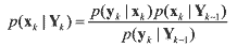 (1) (1)The Chapman-Kolmogorov prediction equation is introduced by
 (2) (2)where xk is the state of interest at time k, yk is an observation taken of this state at time k, and
For most applications, however, closed-form solutions of the posterior update equation
III. SUBOPTIMAL NONLINEAR FILTERINGThis section illustrates the integration of the proposed adaptive filtering algorithms with the
sigma point filters (SPFs)21, such as UKF and DDF, for more enhanced nonlinear filtering
algorithms. Thus, the adaptive sigma point filters (ASPFs) lead to the adaptive unscented
Kalman filter (AUKF) and the adaptive divided difference filter (ADDF). The objectives of
the integrated adaptive nonlinear filters are to take into account the incorrect time-varying
noise statistics of the dynamic systems and to compensate for the nonlinearity effects
neglected by linearization.
1. Adaptive Unscented Kalman FilteringThe unscented Kalman filtering8 algorithm is summarized for discrete-time nonlinear equations
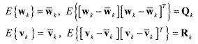
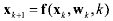 (3) (3)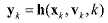 (4) (4)where xk Є Rn is the n×1 state vector and yk Є Rm is the m×1 measurement vector at
time k. wk Є Rq is the q×1 process noise vector and vk Є Rк is the r×1 additive
measurement noise vector, and they are assumed to be zero-mean Gaussian noise processes
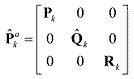
with unknown covariances given by Qk and Rk respectively. The original state vector is redefined as an augmented state vector xak along with noise variables, and an augmented covariance matrix Pak on the diagonal is reconstructed
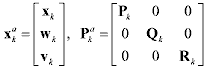 (5) (5)where na = n + q + r is the dimension of the augmented state vector. Then, a set of the scaled symmetric sigma points
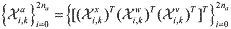 is constructed is constructed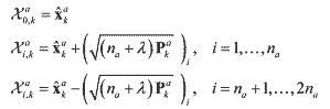 (6) (6)where λ = α2(na + κ) - na includes scaling parameters. α controls the size of the sigma point
distribution and should be a small number (0 ≤ α ≤ 1) and κ provides an extra degree of
freedom to fine tune the higher order moments κ = 3 - na for a Gaussian distribution.
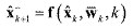
 is the ith column or row vector of the weighted square root of the scaled covariance matrix (na + λ)Pak. is the ith column or row vector of the weighted square root of the scaled covariance matrix (na + λ)Pak.As for the state propagation step, the predicted state vector
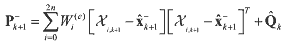
 and its predicted covariance P-k+1 are computed using the propagated sigma point vectors. and its predicted covariance P-k+1 are computed using the propagated sigma point vectors. (7) (7) (8) (8) (9) (9)where Χxi,k is a sigma point vector of the first n elements of the ith augmented sigma point
vector Χai,k and Χwi,k is a sigma point vector of the next q elements of ith augmented sigma
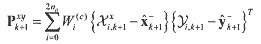
point vector Χai,k, respectively. Similarly, the predicted observation vector
 and the
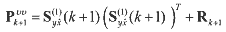
innovation covariance Pυυk+1 are calculated and the
innovation covariance Pυυk+1 are calculated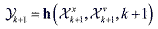 (10) (10)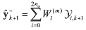 (11) (11)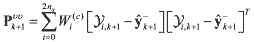 (12) (12)where Χνi,k is a sigma point vector in the r elements of the ith augmented sigma point
vector Χai,k. Wi(m) is the weight for the mean and Wi(c) is the weight for the covariance given by
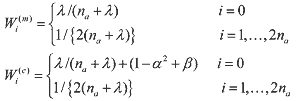 (13) (13)where β is a third parameter that further incorporates higher order effects by adding the
weighting of the zeroth sigma point of the calculation of the covariance, and β = 2 is the
optimal value for Gaussian distributions. Now, the Kalman gain Κ(k+1) is computed by
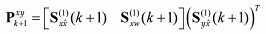
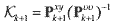 (14) (14)and the cross correlation matrix is determined
 (15) (15)The estimated state vector
 and updated covariance P+k+1 are given by and updated covariance P+k+1 are given by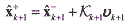 (16) (16)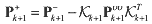 (17) (17)where
 is the innovation vector that is the difference between the observed measurement vector and the predicted measurement vector. is the innovation vector that is the difference between the observed measurement vector and the predicted measurement vector.Note that for implementing the proposed adaptation algorithm into the SPFs the
expression of the process noise covariance matrix in the predicted covariance equation should
be explicit. However, the process noise covariance term in the UKF algorithm is implicitly
expressed in the predicted covariance equation, thus, the noise adaptive estimator cannot be
directly implemented.
There are two approaches that can integrate the proposed adaptive algorithm into the
unscented Kalman filtering21. The first method is to use the augmented covariance matrix Pak given in Eq. (15), where the current process covariance matrix Qk is replaced with the estimated covariance Q^k and at each time step new sigma points drawn from the new augmented covariance matrix P^ak are used for the propagation step.
 (18) (18)The second approach uses the assumption that both the process and measurement noises
are purely additive. Then, the sigma point vectors Χwk and Χνk for the process and
measurement noise are not necessary, and the sigma point vector reduces to Χak = Χxk ≡ Χk.
Thus, the process noise covariance can be expressed explicitly in the predicted covariance
equation as
 (19) (19)Now, the noise adaptation estimator can be directly applied to formulate an adaptive
unscented Kalman filter algorithms. From Maybeck’s unbiased adaptation algorithm22, the
observation of the process noise matrix was rewritten as the difference between the state
estimate before and after the measurement update
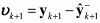
 (20) (20)where the term qk ≡ Κkvk is the state residual and represents the difference between the state estimates before and after the measurement update. Q^-k ≡ Qk is the current expected process
noise covariance. If the residual has a large value, then it indicates that the future state
prediction is not accurate enough. The first term in the above equation is a measure of the
state residual, and the next term is a measure of the correction in the expected change of
covariance. It is rewritten and becomes obvious conceptually
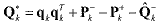
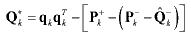 (21) (21)The equation shows that Q•k is the residual minus the change in the a posteriori covariances between two consecutive time steps.20 The measure of the process noise Q•k is then combined with the current estimate Q^-k in a moving average
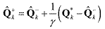 (22) (22)where γ is the window size that controls the level of expected update change and needs to be selected through a trial-error method. If γ is small, then each update is weighted heavily, but
if γ is large, then each update has a small effect. The performance of the adaptive routine is
very sensitive to the selection of γ, and thus should be selected for each application.
Denote Qk ≡ Q^+k, then the estimated covariance matrix is used in the covariance propagation step in Eq. (18). Now, the discrete formulation is placed into a continuous form. If the
estimated discrete-time process noise covariance matrix is written by
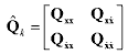 (23) (23)then diagonalization of the process noise covariance of the velocity part can be made
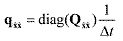 (24) (24)Now the continuous process noise covariance update is redefined as
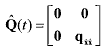 (25) (25)This updated estimate Q^(t) is used for the state propagation between time-step t and t+dt.
Note that the proposed adaptive algorithms highly depend on the selection of the weight
factor γ. In order to provide the consistent, optimal performance of the proposed adaptive
filter, we suggest an efficient calibration method in this paper. Now the question comes to
mind is how the scaling factor γ should be determined. The brute-force way for computing
the scale factor is to use the trial-error approach until the filter produces a sub-optimal or
near-optimal estimation result. In this paper, an efficient derivative-free numerical
optimization technique is utilized for automated calibration of the weight scale factor. The numerical optimization method called the Downhill Simplex algorithm21 is used to tune the
parameters of the process noise covariance. In order to apply the numerical optimization
algorithm to the filter tuning, the tuning problem must be expressed by a numerical
optimization or function minimization problem. The objective function is constructed in terms
of the innovation vector concept instead of the estimate error. To obtain an on-line optimal
estimator it is assumed that the system noise was slowly varying over Ns time steps. The cost
function is expressed as follows
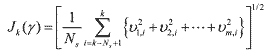 (26) (26)where υm,i is each component of the innovation vector, Ns is the number of time steps, and m is the dimension of the observation vector. The objective of the optimization is to find a optimal weight parameter γopt such that it minimizes the sum of the innovation errors or the state errors. The weight scale factor can also be obtained off-line by making use of the cost
function including all the innovation errors over the entire estimation period.
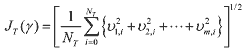 (27) (27)where NT is the total number of time steps over the entire estimation period. Note that in the off-line method if the initial innovation vectors contain large errors it is necessary to neglect
them in the cost function because large initial innovation errors make the estimator converge
slowly.
2. Adaptive Divided Difference FilteringIn this section, the proposed noise estimator algorithm is combined with the divided
difference filter (DDF)9 such that the integrated filtering algorithm leads to the adaptive
divided difference filter (ADDF). The first-order divided difference filter (DDF1) is
illustrated for general discrete-time nonlinear equations with the assumption that the noise
vectors are uncorrelated white Gaussian processes with unknown expected means and
covariances
 (28) (28)First, the square Cholesky factorizations are introduced
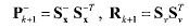
 (29) (29)The predicted state vector x^-k+1 and the predicted state covariance P-k+1 are computed
 (30) (30)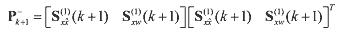 (31) (31)where
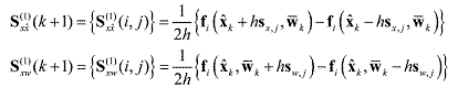 (32) (32)where sx,j is the column of Sx and sw,j is the column of Sw from Eq. (29) . Next, the square
Cholesky factorizations are performed again
 (33) (33)The predicted observation vector y^-k+1 and its predicted covariance are calculated in a similar fashion
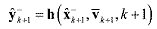 (34) (34)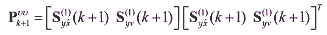 (35) (35)where
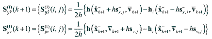 (36) (36)where s-x,j is the column of S-x and sv,j is the column of Sv. If the measurement noise vector is simply additive, then the innovation covariance Pυυk+1 is computed as
 (37) (37)Finally the cross correlation matrix is determined by using
 (38) (38)In the update process, the filter gain Κk+1, the estimated state vector x^+k+1, and updated covariance P+k+1 can be computed by using the same formulas as in the UKF.
For the adaptive divided difference filter formulation, the method used to combine the
proposed noise estimator with the DDF is to just perform the square Cholesky factorization
sequentially at each time when the estimated covariance is updated from the noise adaptation.
If the estimated covariance matrix in Eq. (22) is factorized at each time
 (39) (39)then, the factorized value is delivered back to the DDF algorithm leading to adaptive filtering
structure.
3. Sigma Particle FilteringIn this section a new particle filtering method, which is based on the bootstrap filter11 and a
new sigma particle sampling method, is illustrated. The new particle filter is called the sigma
particle filter. In this section, a specific algorithm for the sigma particle filter (SPF) is
explained. The implementation of the sigma particle filter consists of three important
operations; 1) prediction of sigma particles, 2) update of the particle weights with
measurements, and 3) drawing sigma particles.
A. Initial SamplingThere are two different ways in which initial sigma particles are drawn23. In this paper, the first method, called the simplified sigma particle sampling method (SSPS), is illustrated. The
particle sampling method yields
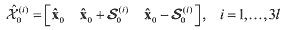 (40) (40)where x^0 is the initial estimate. The second option is to use the random sampling used in the particle filtering from either a Gaussian distribution or uniform distribution
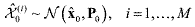 (41) (41)where M is a larger number than that of N in the sigma particles, (M >> N). Even though M random samples are used in the prediction at the next step, the number of samples is reduced to N in the update procedure by adopting the sigma particle sampling method.
B. PredictionThe prediction of the drawn samples is performed by using the system dynamic function in
the same way as the particle filtering
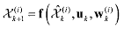 (42) (42)where w(i)k are the N samples of the process noise drawn by w(i)k ~ p(wk).
C. UpdateThe important weights are updated by selecting the important function as the state
propagation density q(xk+1|Xk, Yk+1)=q(xk+1|xk), which yields
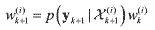 (43) (43)where the likelihood probability density p(yk+1|Χ(i)k+1) is computed by
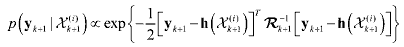 (44) (44)and Rk+1 is an exponentially time-varying measurement noise covariance matrix, which plays an important role of adjusting the variance of the likelihood function. The idea of this time-
varying measurement covariance matrix is to adjust the likelihood function so that particles
with high important weights can be produced. Let the initial measurement covariance matrix
Rk be multiplied by a scale factor λs, and denote R0=λsRk. Then, the exponentially time-
varying measurement noise covariance Rk+1 is computed by
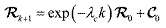 (45) (45)where λc is a time constant controlling the decaying rate, λs is a scale factor adjusting the size of the measurement noise variance, C0 is a constant tuning matrix, and k is the discrete-time index. Note that it is necessary to tune the constant parameters to produce the best estimate results. If necessary, the total simulation period can be divided into sections, and a different exponentially time-varying measurement covariance matrix Rk+1 can be applied to each corresponding section. The updated weights are normalized for the next time step
 (46) (46)Now, an estimate of the current mean value and covariance is obtained by
 (47) (47) (48) (48)where w(i)k+1 are the normalized weights in the update step, and the state samples x(i)k+1 are obtained in the prediction step. Now, it is necessary to update the sigma particles from the estimated mean and covariance by using either the GSPS or SSPS method23. Applying the SSPS method yields
 (49) (49)Then, newly sampled particles are fed back to the prediction step.
SIMULATION RESULTSThe criteria for judging the performance of the proposed adaptive filters are the magnitude of the residuals and their statistics. If the measurement residuals or the state estimation errors are
sufficiently small and consistent with their statistics, then the filter is trusted to be operating
consistently. In other words, the most common way for testing the consistency of the filtering
results is to depict the estimated state errors with the 3-sigma bound given by
 . If the errors lie within the bound, the estimation result is believed to be consistent and reliable.
Instead of the state estimation errors, the measurement innovation vector can be also used for
the filter performance analysis. If the measurement residuals lie within the 2-sigma bound, . If the errors lie within the bound, the estimation result is believed to be consistent and reliable.
Instead of the state estimation errors, the measurement innovation vector can be also used for
the filter performance analysis. If the measurement residuals lie within the 2-sigma bound,  , it indicates the 95% confidence of the estimation results. , it indicates the 95% confidence of the estimation results.1. Orbit Estimation ExampleThe performance of the proposed adaptive nonlinear filters, the AEKF, AUKF, and ADDF is demonstrated through simulation examples using realistic satellite and observation models.
The satellite under consideration has the following orbit parameters: a = 6978.136km, e = 1.0×10⁻⁵, i = 51.6°, ω = 30°, Ω = 25°, E = 6°. The system dynamic equations consist of the two-body motion, J2 zonal perturbation and drag perturbation. The ballistic parameter
taken is B* = 1.0×10⁶ kg/km2 where the drag coefficient has Cd = 2.0. All dynamic and matrix differential equations are numerically integrated by using a fourth-order Runge-Kutta algorithm.
One ground tracking site was used to take observations and the location of the sensor
was selected to be Eglin Air Force Base whose location is at 30.2316° latitude and 86.2147°
longitude. Each observation consists of range, azimuth and elevation angles, and the
measurement errors are considered to be Gaussian random processes with zero means and
variances
 (50) (50)Observations are available from two widely separated tracks. Thus the estimated state
and covariance matrix from the first track are propagated up to the next available
measurements. The second track has some uncertainty as well as nonlinearity due to the
propagation from the end of the first track. Each track length is 2~3 minutes with observations
at every 5 seconds. Visibility of the satellite is decided by checking the elevation angle (EL).
If EL is less than 10°, prediction is performed until the next available observation with EL
greater than 10°. Once EL crosses the threshold boundary, estimation begins and the
estimation mode continue during the 2~3 minutes.
The state vector for the UKF is augmented with the process noise terms wk,
 . The parameters used in the UKF are the scaling factors associated with the scaled unscented transformation. β = 2 is set to capture the higher order (fourth)
terms in the Taylor series expansion, κ = 3 - nα is used for multi-dimensional systems, and
α = 10-3 is chosen to be small in order to make the sample distance independent of the state
size. The interval length h = √3 is set for a Gaussian distribution in the DDF. . The parameters used in the UKF are the scaling factors associated with the scaled unscented transformation. β = 2 is set to capture the higher order (fourth)
terms in the Taylor series expansion, κ = 3 - nα is used for multi-dimensional systems, and
α = 10-3 is chosen to be small in order to make the sample distance independent of the state
size. The interval length h = √3 is set for a Gaussian distribution in the DDF.First Track EstimationThe “solve-for” state vector xk consists of the position, velocity, and drag coefficient, x = [x,y,z,x•,y•,z•,Cd]T . The true initial values of the state variables were
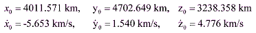 (51) (51)and the drag coefficient was Cd = 2.0. For the nominal reference trajectory, the following initial estimates were used
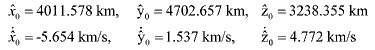 (52) (52)and the initial estimate of the drag coefficient was C^d = 3.0. The initial covariance P0 є R7×7 used for the filters had diagonal elements
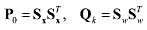
 (53) (53)Often, the process noise for the dynamic model errors is added to the acceleration terms
to help adjust the convergence properties. In this study, however, the value for Q(t) is set,
rather than adjusted, in order to model the realistic environment as close as possible. For instance, the acceleration due to J2 is approximately 10-5 km/sec2 , and the truncated or
ignored perturbing accelerations are roughly of order J22. Therefore, in the orbit model, the
process noise matrix takes the values
 (54) (54)Note that since the process noise covariance Q(t) comes from a continuous-time dynamic system model, it is necessary to convert it into the discrete-time form of the
covariance Qk through an approximate numerical integration scheme1, that is, QkQ(t)Δt,
where Δt is the time step.
For establishing accurate estimation conditions a few measurements were utilized to
produce an initial orbit determination of the state of the satellite. The initial state estimation
was executed by employing the Herrick-Gibbs algorithm24 as a batch filter such that it is
assumed that the conditions for sub-optimality or near-optimality of the filters are satisfied in
the first track. Therefore, in the first track the performance of the three nonlinear filters EKF,
UKF, and DDF are compared without integration of the nonlinear adaptive estimator.
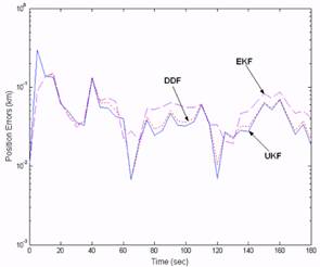
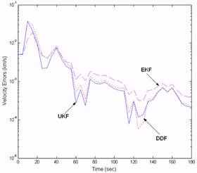
The absolute magnitude values of the position and velocity errors for the three
nonlinear filters are shown in Figures 1 and 2, respectively. As can be seen, the advantage of
the SPFs over the EKF in the position and velocity estimation errors is not obvious, but the
SPFs are slightly better, which indicates that the effect of nonlinearity on the filters is not
severe with the small initial state errors along with the small process noises over the short
track length.
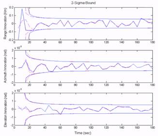
Fig. 3 shows the measurement innovation errors that lie inside the 2-sigma bound
without any deviations. Even though each filter produces slightly different innovation errors,
they all fall inside the boundary with close optimal performance. According to the criteria
such as the RMS errors, and the innovation error, it is seen that the performance of the
nonlinear filters is near-optimal when the process and measurement noise are correctly selected but the SPFs are slightly better than the conventional EKF due to the neglected nonlinear effect.
Second Track EstimationThe second track was separated from the first track by approximately 24 hours. Due to the
long propagation time large state errors occur. During the prediction period between the first
and second tracks, each propagation method in the filters was used in order to propagate the
estimated state and covariance matrix. Thus, the inputs to the orbit determination in the
second track are the a priori state estimate and covariance matrix propagated from the end of
the first track, and each nonlinear filter has the same initial state and covariance values. The
prediction equations used consist of the two-body motion, J2 zonal perturbation and drag
perturbation, but no process noise was added on it.
There are two factors that affect the accuracy of the second track estimation, the
separation time and the first track length. As the separation time between tracks increases the
prediction errors increase due to the neglected nonlinear terms in the prediction process,
which affects the estimation in the second track. Also, large errors could occur even if the
system was linear because a 3-minute 1st track does not allow an accurate state estimate. The
uncertainties or neglected modeling errors in the second track, however, can be compensated
for by utilizing the proposed adaptive nonlinear filtering techniques that adaptively estimate
the process noise covariance matrix. Thus, the purpose of the orbit estimation in the second-
track is to compare the performance of the proposed adaptive nonlinear filters, AEKF, AUKF
and ADDF with the standard nonlinear filters.
The true initial values of the state variables for the second track estimation had the
following
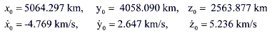 (55) (55)and the drag coefficient was set Cd = 2.635. For the nominal reference trajectory, the initial estimates for the second track estimation were used
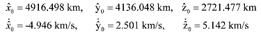 (56) (56)and the initial estimate of the drag coefficient was C^d = 3.0. The process noise covariance matrix used was the same as the first track, except the variance value of the drag coefficient
was increased in order to consider uncertainty effects due to the propagation.
 (57) (57)The adaptive nonlinear filters used for the state and parameter estimation are based on
the identification of the process noise Q(t). Since each adaptive filter produces a different
value of the objective function J that is the sum of the innovation errors, the weight factors
calibrated from the Downhill Simplex optimization method are different. The weight factor or
wind size γ for the AEKF was 4.5×10⁵, the values for the AUKF and ADDF were
approximately equal with γ = 1.65×10².
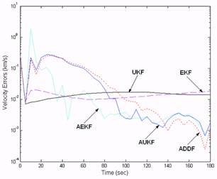
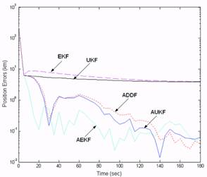
Figures 4 and 5 are the plots of the performance comparison of the adaptive filters and
nonlinear filters with respect to the position and velocity estimation errors in the second track,
respectively, which illustrate a possible realistic scenario in orbit determination. From the
previous simulation results in the first track, it is expected that the UKF performance should
be superior to the EKF performance. However, the UKF results of the averaged magnitudes of
the position and velocity estimation errors are very close to those of the EKF with the biased
estimation errors. The degradation of the EKF and UKF performance is related to the fact that
the state and covariance prediction executed for a long-time interval leads to large prediction
errors due to the effects of the neglected nonlinear terms, the parameter uncertainties such as
the drag coefficient, and also the initial errors from the 1st track. Thus, the filters start
estimating the states with large initial state errors and large covariance matrices with
unknown statistical information of the uncertainties or noise. Under the incorrect noise
information, even the UKF or higher-order nonlinear filters can’t produce optimal estimates
due to the violation of the optimality conditions. On the other hand, all the adaptive filters
(AUKF, ADDF and AEKF) converge continuously and fast with small bias error, which
indicates they are performing in a near optimal fashion. The performance in the velocity estimation also shows that the adaptive nonlinear filters provide a more accurate estimate than
that of the standard nonlinear filters (the EKF and the UKF). This agrees well with our
expectations and indicates that the correct noise information is necessary for the filters to
perform optimally.
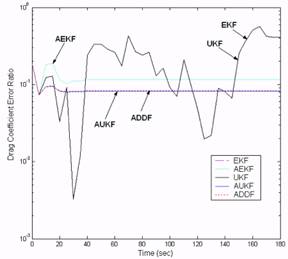
In Fig. 6 the absolute values of the drag coefficient error ratio with respect to the
proposed adaptive filters are shown in the available second track, where the error ratio is the
ratio between the true and estimated drag coefficient. As expected the parameter estimation
with the adaptive filters also successfully generated converged solutions with the fast and
accurate estimates. The EKF and UKF also converge, but with large bias errors. In the drag
coefficient estimation, the AUKF and ADDF show better performance over the AEKF.
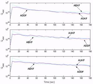
Fig. 7 illustrates the adaptation of the process noise variance generated from the
adaptive nonlinear filters. It is seen that while the manually-tuned covariance is constant with
time, the estimated covariance has time-varying values that are continuously estimating and
adapting the noise statistics for an optimal performance. From the results it is seen that the increased process noise variances at the initial estimation make the prediction covariance and
the Kalman gain bigger, therefore the observations have much influence on the filters. In
contract as the variances decrease with time, the Kalman gain becomes small and then the
effect of the observations on the filters is reduced. For optimal performance of the filters the
process noise variance might be required to increase from the initial variances.
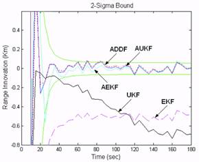
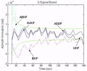
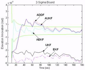
Fig. 8 (a)-(c) depicts the innovation errors with the 2-sigma bound. The innovation
errors from the adaptive filters vary inside the sigma bound, but the innovations from the EKF
and UKF are outside the bound. According to these results, we can also judge that the
adaptive filters achieved the near-optimal performance.
According to the criteria of the RMS errors, the nonlinearity index, and the innovation
error presented so far, it is seen that the performance of the adaptive nonlinear filters is
optimal in the sense that they compensate for the neglected modeling errors as well as the
unknown uncertainties.
2. Falling Body Tracking ExampleIn this section the performance of the sigma particle filter algorithm is demonstrated and
compared with the nonlinear Gaussian filters including the extended Kalman filter (EKF), the
unscented Kalman filter (UKF), and divided difference filter (DDF). To test the performance
of the proposed nonlinear filters the vertical falling body example described in Fig. 9 is used
because it contains significant nonlinearities in the dynamical and measurement equation.
This falling body example originates from Athans, Wishner, and Bertolini [24], and has
become a benchmark to test the performance of newly developed nonlinear filters. For
instance, the UKF algorithm [8] and the DDF [9] were tested and compared with the Gaussian
second-order filter as well as the EKF. See Ref. 25 for additional applications of the nonlinear
filters.
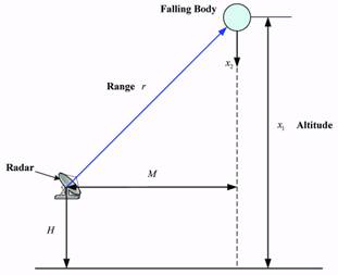 Fig. 9. Geometry of the Vertically Falling Body.
The goal of the nonlinear filtering is to estimate the altitude x1, the downward velocity x2, a constant ballistic parameter x3 of a falling body that is reentering the atmosphere at a very high altitude with a very high velocity. The radar measures the range rk which is updated each second and corrupted with additive white Gaussian noise νk which has
zero mean and covariance E{νkνkT} = Rk. The trajectory of the body can be described by the
first-order differential equations for the dynamic system
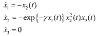 (59) (59)The radar, located at a height H from the mean sea-level and at a horizontal range M from the body, measures the range rk, which is corrupted by Gaussian measurement noise νk
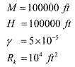
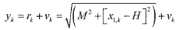 (60) (60)where νk is the measurement noise represented with zero-mean and covariance Rk. The measurements are made at a frequency of 1 Hz. The model parameters are given by
 (61) (61)and the initial state x0 of the system is
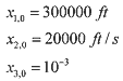 (62) (62)The a priori state estimate x^0 is given by
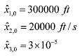 (63) (63)and covariance matrix P0 is selected as
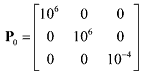 (64) (64)Process noise was not included in the trajectory simulation, therefore Qk = 0. For the numerical integration of the dynamic differential equations small time steps are required due
to high nonlinearities of the dynamic and measurement models. A fourth-order Runge-Kutta
scheme with 64 steps between each observation is employed to solve the first-order
differential equations. For the UKF κ = 0 was chosen in accordance with the heuristic
formula na+κ = 3, and h = √3 was used in the DDF. For sigma particle generation in the SPF, the simplified sampling method in Eq. (39) was used. The total number of sigma
particles generated was N=91, which is larger than that of the UKF but much smaller than that
in the particle filter (usually N is larger than 300 or 1000 in particle filtering). The initial
estimates or mean values used in the initial sigma particle sampling step are assumed to be the
true values, x0 = x^0. The constant parameter values used for the sigma particle sampler in the SPF were l = 3, τ = 0.1, and 1. The tuning parameters used for the exponentially time-varying measurement noise covariance are λc = 0.023, λs = 10-3, C0 = 0.
The performance of the nonlinear filters is compared in terms of the average root mean
square error, which is defined by
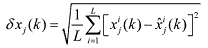 (65) (65)where L is the Monte Carlo simulation run, and subscript j denotes the j-th component of the vector x(k) and its corresponding estimate x^(k), and the superscript i denotes the i-th simulation run. To enable a fair comparison of the estimate produced by each of the four filters, the estimates are averaged by a Monte Carlo simulation consisting of 30 runs.
In Fig. 10 the average magnitude of the position error is depicted by each filter. As can
be shown, the performance of the SPF dominates the nonlinear Gaussian filters. The error of
the SPF is smaller than the others, and more importantly, the convergence of the estimation of
the SPF is much faster than those of the other filters, which is a very encouraging factor for
the filter performance. The velocity estimates are shown in Fig. 11 where large peak errors
occur in the nonlinear filters, but the SPF recovered quickly and had a smaller peak error. The
UKF had smaller errors than the EKF and DDF, but a larger peak error. This spike motion
occurred when the radar range was perpendicular to the trajectory and, as such, it didn’t
provide enough measurement information to the filters. Fig. 11 shows the SPF can work
correctly in a situation where there is not enough measurement information.
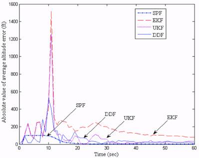 Fig. 10. Absolute Errors in Position Estimate.
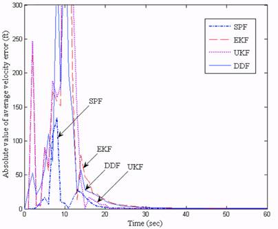 Fig. 11. Absolute Errors in Velocity Estimate.
Fig. 12 indicates the errors in estimating the ballistic parameter. The error from the SPF
converged quickly to a value very near zero. It shows that the SPF performs better than the
EKF and higher-order nonlinear filters. In addition, the performance of the DDF is slightly
better than the UKF, but much better than the EKF. The difference of the estimate results
between the UKF and DDF is not as dramatic, but they exhibited larger errors than the SPF.
In addition, the figures show that the SPF produced nearly unbiased optimal estimates.
Fig. 12. Absolute Errors in the Ballistic Coefficient Estimate.
CONCLUSIONSIn this paper new nonlinear filtering algorithms called the adaptive unscented Kalman filter,
the adaptive divided difference filter, and the sigma particle filter are utilized to obtain
accurate and efficient estimates of the state as well as parameters for nonlinear systems with
unknown noise statistics. The purpose of the adaptive nonlinear filtering methods is to not
only compensate for the nonlinearities neglected by linearization, but also to adaptively
estimate the unknown noise statistics for optimal performance of the filters. The sigma
particle filtering algorithm can be used for nonlinear and/or non-Gaussain state estimation.
Simulation results indicated that the performances of the new nonlinear Bayesian filtering
algorithms are superior to the standard nonlinear filters, the extended Kalman filter, the
divided difference filter, and the unscented Kalman filter in terms of the estimation accuracy
of states and parameters and robustness to uncertainties. In particular, the robustness of the
adaptive filters to the unknown covariance information provides the flexibility of
implementation without the annoying manual-tuning procedure. In addition, the sigma
particle filters can dramatically reduce the computational complexity of a particle filtering
implementation by employing an efficient sampling approach called the deterministic sigma
particle sampling method. The advantages of the proposed adaptive nonlinear filtering
algorithms make these suitable for efficient state and parameter estimation in not only satellite
orbit determination, but also other application areas.
REFERENCES
Размещен 24 декабря 2006.
| ||||||||||||||||||||||||||
|
|
|
|
|
|
|
|