


|
|
|
|
|
|
|
|
ON A NEW VERSION OF THE ORBIT DETERMINATION METHODAlla S. SochilinaCentral Astronomical Observatory at Pulkovo, St.-Petersburg, Russia Rolan I. Kiladze Abastumani Astrophysical Observatory, Republic of Georgia, FSU
1. THE METHOD OF DETERMINATION OF PRELIMINARY ORBITSAt present a great number of the faint fragments have been discovered in the vicinity of the
geostationary orbit (GEO), and they are to be catalogued [1].
The observations of geostationary objects (GO) made over short time-intervals, permit,
as a rule, determining only circular orbits. The principal difficulty of the calculation of an
elliptical orbit by Gauss’s method consists in finding topocentric distances (ρ).
The determinant (DD) of the system of equations for the case of N observations can be expressed in the form
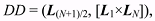 (1) (1)where Lj is the unit vector (cosαj cosδj, sinαj cosδj, sinδj).
If DD is equal to 10-6 ÷ 10-5 , then the accuracy loss will be close to 5-6 digits;
especially, in the following orbital elements: the semi-major axis (a), the eccentricity (e), and
the argument of the perigee (ω). So the value of DD can be used as an indicator of the
resulting reliability.
However, the preliminary values of topocentric distances can be calculated by using
both the orbital inclination (i) and the longitude of the ascending node (Ω) of the circular
orbit, and the conditions [2]:
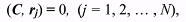 (2) (2)where C = (sini sinΩ, –sini cosΩ, cosi) is the unit vector perpendicular to the orbital plane, and rj, the vector of the geocentric distance of the object for the time-moment tj of observation. This is expressed as follows:
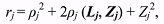 (3) (3)or
 (4) (4)where Zj is the geocentric vector of an observatory with coordinates (Xj, Yj, Zj), calculated for
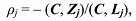
corresponding time-moments tj. Then the equation for ρj can be obtained by multiplying equation (3) by the vector С and taking into account (2):
 (5) (5)By use of formulae (3) (5) the geocentric rectangular coordinates xj, yj, zj of GO for each time-moment of observations, the distances rj and the arguments of latitude uj = νj + ω
(where νj is the true anomaly) can be computed by use of the formulae of the two-body-
problem. The obtained rj and uj can be represented by Taylor series as follows:
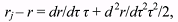  (6) (6)where r and u denote the values of rj and uj for the initial moment of time t0, and τ = GM (t–t0)
(GM = 107.08828 in terms of the constants adopted for the GO).
The analytical representations of the derivatives in terms of the orbital elements are
given as follows:
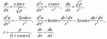 (7) (7)It should be noticed that for circular orbits the first derivatives dr/dτ = 0 and
(du/dτ) 3r = 1, but the second derivatives are close to their exact values. Taking into account
the analytical expressions (7) of the derivatives, the following expression
 (8) (8)can be used in the second approximation instead of dr/dτ.
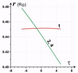
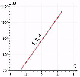
The equation (8) allows organizing the iteration process, which is shown in Figs. 1 and 2.
After calculating more precise rj and uj in the second approximation all orbital elements
are determined. The main idea of the method is to achieve an agreement between the
elements, which are calculated from the geometry (by use of rj), and those from the dynamics
(by use of uj).
2. THE CHECK CALCULATIONSTo check the method the model observations have been generated using the GO 68081E
fragment data obtained by V. Biryukov and V. Rumyantsev at the Crimean observatory. From
the beginning its orbit was improved, all perturbations being taken into account, by use of the
observations for October 18, 2004, distributed over the 160 minute time interval. After that
the ephemerides were calculated for 69 points with the step of 2 minutes, taking into account
the secular perturbations only.
In Table 1 in the first line the improved values of the orbit elements are given. In the
second line the elements of the preliminary orbit are shown, calculated by the new method, by
use of all 69 model observations. The determinant of the system DD = 0.003571, and the
obtained orbit slightly differs from the initial one, representing the model observations to the
precision of 0”.06.
Table 1. The elements of preliminary orbits, calculated by use of the model observations.
The representation errors for the model observations on short time-intervals are smaller
than 0”.1. The errors of representation by means of circular orbits are 1-3”.
In Table 2 eight orbits are shown as calculated on the short time-interval by use of the
same observations.
Table 2. Preliminary orbits calculated by use of model observations over the short time
intervals (?t = 16 minutes) and with the determinants DD, which are 0.579015x10⁻⁵ through
0.609425x10⁻⁵.
The errors of representation of the model observations on these short time-intervals are
smaller than 0”.2. The errors of representation by means of circular orbits are 1-3”.
In Table 3 the preliminary orbits of GO 90003 are shown as having been calculated by
use of the real observations for different time-intervals, their different distributions being
given. The letter “с” means a circular orbit and “е” means an elliptic one.
In the first case the determinant DD = 0.17063x10⁻⁵ and the precision of the observations is 10 times worse than in the case of the model observations. Therefore, the
values of elements e, ω and n (the mean motion of the object) differ from the check orbit, and
it is necessary to extend the time-interval in order to increase the precision of these elements.
Table 3. Preliminary orbits calculated by use of the real observations of GO 90003.
3. CONCLUSIONSIn conclusion it should be noted that the suggested method of orbit determination for the
geostationary objects permits achieving, as compared with classical methods, a better
precision on the short time-interval.
Acknowledgements. This research is supported by the Grant of INTAS-01-0669.
REFERENCES
Размещен 6 декабря 2006.
| |||||||||||||||||||||||||||||||||||||||||||||||||||||||||||||||||||||||||||||||||||||||||||||||||||||||||||||||||||||||||||||||||||||||||||||||||||||||||||||||||||||||||||||||||||||||||||||||||||||||||||||||||||||||||||||||||||||||||||||||||||||||||||||||||||||||||||||||||||||||||||||||||||||||||||||||||||||||||||||||||||||||||||||||||||||||||||||||||||||||||||||||||||||||||||||||||||||||||||||||||||||||||||||||||||||||||||||||||||||||||||||||||||||||||||||||||||||||||||||||||||||
|
|
|
|
|
|
|
|