


|
|
|
|
|
|
|
|
DRAG COEFFICIENT VARIABILITY AT 175-500 KM FROM THE ORBIT DECAY ANALYSES OF SPHERESBruce R. Bowman*Air Force Space Command, Space Analysis Division/XPY, Kenneth Moe Science and Technology Corp.
INTRODUCTIONThe US Air Force has long supported efforts to improve satellite orbital predictions, in
cooperation with the US Navy, NASA, the Harvard-Smithsonian Center for Astrophysics, and
many universities and Air Force contractors. Over the years, the Air Force prediction efforts
have evolved along two lines: (1) In the High Accuracy Satellite Drag Model (HASDM)1
program many orbiting satellites are used to monitor the atmosphere and update an
atmospheric model in real time; (2) In the DMSP Program, the spectroscopic sensors SSUSI
and SSULI will monitor the atmosphere and update it. A major objective of both these
programs is to measure and predict absolute atmospheric densities. Improvement in the
knowledge of drag coefficients contributes directly to that goal.
Better drag coefficients will also contribute to the improvement of thermospheric
density models. A landmark in the effort to improve models was achieved by Marcos2 in
1985 when he compared and evaluated 14 models against accelerometer measurements from
seven satellites. A decade later, Chao et al3. used orbital data from the ODERACS I and
ODERACS II families of spheres to measure the biases in the Jacchia 71 and the MSIS 90
density models near sunspot minimum. They accomplished this by comparing the fitted drag
coefficient, CD, with the physical drag coefficient, CDP, calculated from the actual momentum
transfer to the satellite. More recently, Owens4 has revised and improved the Jacchia models
to create the NASA Marshall Engineering Thermospheric Model –Version 2.0 (MET-V 2.0
Model). This model has been subjected to an extensive statistical evaluation by Wise et al5.
Further recent progress6 in the analysis of orbital data has refined the semiannual variation and other parameters of the Jacchia 70 thermospheric density model7. This new
development has presented an opportunity to use the improved Jacchia model with data from
spherical satellites to refine our knowledge of drag coefficients and improve the absolute
densities in the model.
ANALYSIS METHOD FOR FITTED DRAG COEFFICIENTSThe method developed to determine accurate CD values is to obtain accurate ballistic
coefficient (B) values from special perturbation orbit fits using a corrected atmospheric
model. In standard orbit fits the B values, equal to the drag coefficient times the area to mass
ratio (CD A/M), also contain unmodeled density variations from orbit fit aliasing, as well as
contain other variations due to frontal area changes plus CD changes. However, if a corrected
atmospheric model can be used then this removes the aliasing of the unmodeled density
variations into the B variations. The corrected model is based on calibrating the atmosphere
on a daily basis from analysis of daily temperature and density corrections on many satellites
over the time period of interest. Once the atmospheric model has been corrected (on a daily
basis) the model is then used to obtain accurate B values. The resulting B variations can then
be attributed solely to CD variations for spherical satellites which have no frontal area
problems.
ATMOSPHERIC MODEL CORRECTIONSDaily temperature corrections to the HASDM modified Jacchia 1970 atmospheric model have been obtained on 79 calibration satellites for the period 1994 through 2003, and 35 calibration
satellites for the solar maximum period 1989 through 1990. All the “calibration” satellites are
moderate to high eccentricity, with perigee heights ranging from 150 to 500 km. Figure 1
shows the satellites grouped by perigee height and inclination for the 1994-2003 period.
 Fig. 1. Calibration satellite orbits as a function of height and inclination bands.
The daily correction values were obtained using a special energy dissipation rate (EDR)
method8, where radar and optical observations are fit with special orbit perturbations. It has
been shown that using this method results in daily average density values (representing drag
at perigee) accurate to 2-4% during solar maximum conditions. The first step was to correct
the local solar time and latitude equations in the atmospheric model. This was accomplished
by least squares fitting all the daily values over the 1994 through 2003 period, obtaining
corrections as a function of local solar time and latitude for different heights and solar EUV
activity. The next step was to use all the calibration satellites daily temperature corrections,
and on a daily basis, least squares fit the values to form a daily global temperature correction
field as a function of height.
The daily temperature correction equations obtained above were then used in the
modified Jacchia 1970 atmospheric model to compute density values at every integration step
during the orbit fits. To validate the temperature corrections orbit fits were obtained on 7
different validation orbits from 1994 through 2003. The validation orbits were chosen to have
moderate to high eccentricity in order that the perigee heights would remain almost constant
during the entire 10-year evaluation period. B values were obtained from the daily orbit fits,
first without the temperature corrections, and then with the temperature corrections. Standard
deviation (STD) values were then obtained on the B values with and without the corrections.
If the temperature corrections are perfect then the B variations should be very small after
applying the corrections. Table 1 lists the validation satellites with the STD results. The STD
values show a very significant reduction. Note that the STD on the B values for the non-
corrected data corresponds mainly to unmodeled density variations, which increase as the
height increases. This has been observed repeatedly from previous HASDM analyses.
Finally, the significant reduction in B STD values demonstrates the validity of the computed
daily temperature corrections.
Table 1. Validation satellites with standard deviations (STD) of B with and without daily
temperature field corrections dTc. Periods of solar minimum (94-97) and solar maximum
(98-02) are listed separately.
DETERMINATION OF PHYSICAL DRAG COEFFICIENTSThe mathematical models of physical drag coefficient CDP that will be used in this paper were developed by Sentman9,10 and Schamberg11,12 at the beginning of the space age. Sentman’s
model was soon tested when the Air Force flew long cylindrical satellites, beginning in 1960.
Although much of the early work was classified, the large drag coefficients calculated in
Sentman’s 1961 papers were confirmed by the data and analyses eventually published by
Bruce13 and by DeVries et al.14. In 1975, Imbro et al.15 demonstrated the utility of Schamberg’s model for investigating the effect of the angular distribution of reemitted
molecules on the drag coefficient. In 1996 it was shown how the two models could be used
together to calculate the effect of a completely diffuse distribution plus a quasi-specular
fraction on the physical drag coefficients of a sphere and a cylinder16. These two models will be used in the present paper to calculate physical drag coefficients to compare with the fitted
drag coefficients of spheres.
Marcos’ 1985 survey2 compared densities calculated from 14 thermospheric models with measurements by accelerometers aboard three long cylindrical satellites and four
compactly shaped satellites, at an average altitude of about 200 km. There was a systematic
difference of about ten percent between the two types of satellites. By using Sentman’s model
with physical parameters measured in orbit, it was possible to reduce this difference to three
percent17,18, and bring the measurements from both types of satellites to within three percent
of the average density from 11 of the most recent density models. These results increase
confidence that drag coefficients calculated from Sentman’s model, using the parameters
(accommodation coefficient and angular distribution) measured near 200 km, are accurate to
about 3 % for satellites having smooth surfaces of typical compositions. The effects of
unusual surface compositions and surface treatments are investigated in the companion
paper38.
The parameters used in drag coefficient models are the angular distribution of
molecules reemitted from the satellite surface and the energy accommodation coefficient,
which is a measure of the fraction of kinetic energy lost before the molecules are reemitted
from the surface. Near 200 km, accommodation coefficients of 0.99 to 1.00 have been
measured by Beletsky19, and by Ching et al.20, while angular distributions within a few
percent of diffuse were reported by Beletsky19, and by Gregory and Peters21; but at 325 km
near sunspot minimum, Imbro et al.15 measured an accommodation coefficient of 0.86 to 0.88.
We don’t know the amounts of atomic oxygen adsorbed on the satellite surfaces in these
particular cases, but we know from decades of satellite and laboratory measurements that
atomic oxygen adsorbs on satellite surfaces and on nearly any material, and we know that it is
continually adsorbing and desorbing22-27. We know from laboratory measurements that
adsorbed molecules greatly increase the accommodation coefficients28,29. We therefore have
used the atomic oxygen measurements collected in the monograph on the US Standard
Atmosphere, 197630 to extrapolate the accommodation coefficient measurements, which were
mostly made near sunspot minimum, to times of high solar activity, at which time there is
much more atomic oxygen in the thermosphere. We also have used these oxygen
measurements to extend the accommodation coefficients to altitudes above 325 km.
The orbital measurements indicate that at altitudes near 200 km, the molecules are
reemitted diffusely with a high degree of energy accommodation. The energy accommodation
coefficient, α, is defined as
 (1) (1)where Ei is the kinetic energy of the incident molecules, Er is the kinetic energy of the reemitted molecules, and Ew is the energy that the reemitted molecules would have if they
were reemitted at the surface (wall) temperature31.
The analysis of the momentum transfer to the satellite, appropriate for the case of
diffuse reemission, was developed by Sentman9,10. The resulting expression for the physical
drag coefficient of a sphere is
 (2) (2)The parameter s is the speed ratio, defined as the velocity of the incident molecules
divided by the most probable speed of the ambient atmospheric molecules. Vi is the speed of
the incident molecules. Vr is the most probable speed of the reemitted molecules. It is related
to α by
 (3) (3)where Ti is the kinetic temperature corresponding to the incident velocity, and Tw is the temperature of the satellite surface (or wall).
Table 2 is presented to provide insight into the various physical contributions to the
drag coefficient. It was calculated from Sentman’s model, and applies to the case of diffuse
reemission at a time of low solar activity. The first contribution, labeled “incident
momentum”, gives the contribution from the flux of incident particles, ignoring the random
thermal motions of the ambient air. The next column gives the contribution of the random
motion, and the third contribution is the drag caused by the reemission of particles. The final
column gives the physical drag coefficient of a sphere at a time of low solar activity, when the
reemitted particles are assumed to have a completely diffuse angular distribution. Table 2
demonstrates the fact that the physical drag coefficient of a sphere at altitudes near 200 km
must be above 2.00.
Table 2. Contributions to the physical drag coefficient CDP
when reemission is diffuse during sunspot minimum.
At altitudes above 300 km at solar minimum, there is a quasi-specular component of
reemission16 that becomes increasingly important as the altitude increases and the surface
coverage of adsorbed atomic oxygen is reduced27. The effect of this component on CDP is
calculated in the companion paper38. The diffuse and quasi-specular contributions to CDP at
sunspot maximum and minimum are tabulated in the appendix of that paper. These values
will be compared with the fitted drag coefficients, CD, in the figures of the present paper.
CD ANALYSIS OF SPHERICAL SATELLITESThe decayed spherical satellites used in this analysis are listed in Tables 3 and 4, which
include the physical and orbital characteristics.
The ODERACS spheres32 were launched for radar calibration studies and decayed during the solar minimum period of 1994-1995. These small 4” and 6” spheres were
excellent candidates for determining the drag coefficient variations resulting from different
surface characteristics. The Starshine satellites were launched, and also decayed, in the 1999-
2002 solar maximum time period. These satellites were used for optical tracking experiments.
Starshine 1 and 2 had 68% of their surfaces covered by small mirrors, while Starshine 3, twice
the diameter of the other two satellites, had only 30% of its surface made up of small mirrors,
the other 70% covered with black chemglaze polyurethane paint. Also used in the analysis
were three radar calibration Calspheres that decayed during solar maximum times of 1989-
1990. In addition, 7 Russian Taifun radar calibration spheres were used in the analysis. The Taifun Yug class was passive hollow spheres with smooth surfaces. One of them decayed
during solar minimum conditions, the other 3 decayed during solar maximum times of 1989-
1990. The Taifun Type 2 spheres were covered with solar cells to provide power to the active
transmissions for tracking purposes. Three of these satellites also decayed during the 1990
solar maximum period. Since the Taifun Type 2 and the Starshine satellites had numerous
flat plates (mirrors or solar cells) attached to the spherical subsurface they cannot be
considered true spheres from the viewpoint of free-molecular aerodynamics. The final sphere
used was GFZ-1, launched in 1995 and decayed four years later. Its surface included 60 large
recessed mirrors used for laser ranging, and therefore also cannot be considered as a true
aerodynamic sphere.
Table 3. Description of the satellites (non-Taifun), with their orbits, used for the CD analysis.
Table 4. Description of the Taifun radar calibration spheres,
with their orbits, used for the CD analysis.
DETERMINATION OF CD VALUESThe same method used to validate the temperature field was used to compute the B values for the analyses of the decayed spheres. The daily temperature field correction equations were
used in the special perturbation orbit fits to correct the atmospheric model. B values were
then obtained each day using the optimum observation span based on the amount of
observable drag. CD values were then computed from the B values using the size and mass of
each satellite listed in the above table.
ODERACS RADAR CALIBRATION SPHERESThere were two separate launches (releases from the Space Shuttle) in 1994 and 1995 to place a number of radar calibration targets in orbit. This analysis used the three 4” and three 6”
spheres included in the releases.
 Fig. 2. B values of two 4” ODERACS spheres placed in orbit during a 1994 Space Shuttle mission. Satellite 22990 had a polished chrome surface, while 22991 had a sandblasted aluminum surface.
Figure 2 shows the B values obtained after using the daily temperature corrections. The
overall variations of approximately +-6% are the result of the remaining unmodeled density
variations. What is notable is the almost constant difference between the two curves. The
curves are almost identical because both spheres were released at almost the same time into
almost identical orbits. Therefore, any unmodeled density variations will affect both spheres
in the same way. The sandblasted surface appears to have an approximate 2% greater B value
than the polished surface. This is discussed in more detail in a companion paper38.
 Fig. 3. The CD values for the ODERACS 6” spheres, plotted as a function of height.
Figure 3 shows the CD values obtained for the three 6” spheres. The 22994 and 22995 spheres were released in 1994, while the 23471 sphere was released in 1995, a year later.
The 10% to 15% differences between the observed and computed drag coefficients are
very significant. This difference, which is also observed later in the plots of the other spheres,
will be discussed later. Table 5 lists the mean, standard deviation of the mean (Mean Sig),
and % difference from that of sandblasted aluminum.
Table 5. Mean and standard deviation CD values for the 4” and 6” ODERACS spheres. The mean CD difference from the sand-blasted (aluminum) surface is also listed.
STARSHINE SPHERES Fig. 4. Starshines 2 (left) and 3 (right).
The second group of spherical satellites analyzed was Starshines. These three satellites were
partly covered with small (1” diameter) flat mirrors to aid in optical tracking, so the
Starshines are not true aerodynamic spheres. Starshine 1 and 2 were released into a near
circular orbit, in 1999 and 2001 respectively, from the Space Shuttle. Starshine 3 was
launched into a near circular orbit in 2001 from Kodiak Island. Starshine 1 and 2 were the
same size, with approximately 850 1” diameter surface mirrors on a substrate of spun
aluminum, and almost the same mass. Starshine 3 was twice as large in diameter as the other
two, and had approximately 1500 1”diameter surface mirrors and 31 1”diameter laser
reflectors on a substrate covered with black chemglaze polyurethane paint. The mirrors
covered 68% of Starshine 1 and 2, but only 30% of Starshine 3. Figure 5 shows the computed
CD values for Starshine 1, obtained from the orbit fit B values, plotted as a function of perigee
height over the last 100 days before decay.
The observed values are very close to the partly quasi-specular computed drag
coefficient curve, although the observed values are still biased lower than the computed
curves. The three Starshine satellites were expected to have very similar CD values, even
though Starshine 3 was larger and was launched into a higher orbit. Figure 6 shows the plot
of CD values for all three Starshine satellites. The observed values for Starshine 1 and 2 agree, while the larger Starshine 3 CD values are lower than the computed curves by 10% to
15% depending on height. The main reason for the difference between Starshines 1 and 2 on
the one hand and Starshine 3 on the other hand is that 68% of the surfaces of Starshines 1 and
2 were covered by small flat mirrors of circular cross section whereas 30% of the black paint
surfaces of Starshine 3 were covered by the same kind of mirrors. The edges of the mirrors
change the aerodynamic characteristics of the sphere. This is especially true near the edge of
the sphere as viewed by the incident airstream. The CD of Starshine 3 can be adjusted to the
CD of a sphere of black chemglaze polyurethane paint as will be explained in the companion
paper38. The adjusted value of CD is 1.90 which is plotted in Figure 6.
 Fig. 5. Plot of the CD values of Starshine 1 as a function of height over the last 100 days of life.
 Fig. 6. CD values for the Starshine satellites, plotted as a function of height.
The adjusted Starshine CD values for 100% black paint on aluminum also are shown.
TAIFUN RADAR CALIBRATION SPHERESThe Russians have launched many Taifun radar calibration spheres into orbit. One class of
Taifun satellites, designated Yugs, was launched into either 300 km by 1600 km orbits, or
nearly 450 km circular orbits. Four such Yugs were used in this analysis. One of them, 21190
decayed during solar minimum in 1995, and the other three Yugs decayed during solar
maximum in 1989-1990. The Yug satellites are passive and hollow, with a smooth surface.
The second class of Taifuns used in the analysis was the Type 2 active radar calibration
spheres. This class of satellites had almost the identical size and mass of the Yugs, the only
real difference being the surface of the Type 2 satellite was completely covered with solar
cells. Since solar cells are flat plates, the Type 2 “spheres” were not true aerodynamic
spheres. The diameters of the Yugs and Type 2 spheres were 2.000m+-0.010m and 2.007m+-
0.010m respectively, with masses of 750kg+-10kg and 750kg+-30kg respectively33.
Figure 7 shows the CD values computed from the orbit fits of the Yug satellites.
Theoretical curves for the quasi-specular CDP values are shown for solar minimum and solar
maximum conditions. The three Yugs that decayed in the solar maximum 1989-1990 period
have CD values consistently lower than the values observed for 21190, which decayed during
solar minimum year 1995. This is consistent with theory; however, all the CD values are
significantly lower than the computed theoretical values, the same results observed for the
ODERACS spheres described above. Figure 8 shows the CD values observed for the Type 2
spheres. What is significant is the much closer agreement with the theoretical values than the
agreement observed with the Yug spheres. Again, the only difference between the Type 2 and
Yug satellites is that the surface of the Type 2 is completely covered with solar cells. The
results for the Type 2 CD values are much more consistent with the results obtained from
Starshine 1 and 2, which were both 68% covered with mirrors. All these anomalous cases
involved flat mirrors or flat solar cells, so the satellite surface was not strictly spherical.
These results will be discussed later in the discussion section below and in the companion
paper38.
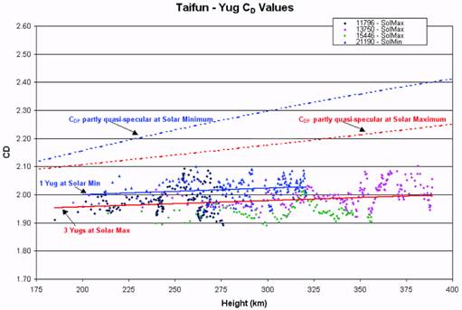 Fig. 7. CD values for Yug true spheres plotted as a function of altitude. Theoretical
partly quasi-specular CDP values are shown for solar minimum and maximum conditions.
 Fig. 8. CD values for three Taifun Type 2 modified spheres are plotted as a function of altitude. Also shown are theoretical CDP values for 100% diffuse and partly quasi-specular conditions.
CALSPHERE RADAR CALIBRATION SPHERESCalspheres 3, 4, and 5 were all launched together in early 1971 into a circular 775 km polar
orbit. They all decayed near the time of sunspot maximum in the late 1989 early 1990 time
frame. King-Hele34 lists the masses as 0.73 kg each, with diameters of 0.26m (10.2”) each.
He also lists the surface as aluminum for Calsphere 3 and 4, and gold for 5. The diameters of
other radar calibration spheres are normally even increments of inches, so it was decided to
use a 10.0” diameter for these spheres. It should be noted that density corrections were
determined for 1989 using approximately 50 satellites that were a subset of the 79 satellites
used for the 1994 through 2003 analyses. Figure 9 is a plot of all three sphere’s CD values as a
function of perigee height. Because of the lightness of the spheres their decay was very rapid
once the perigee height fell below 500 km. Figure 9 represents the decay during the last 100
days of lifetime. There are no data points below 300 km because it took less than 24 hours for
them to decay from a circular orbit of 300 km.
 Fig. 9. CD values for Calspheres 3 through 5, plotted as a function of height
GFZ-1 SPHEREGFZ-1 was a geodetic satellite designed to improve the current knowledge of the Earth’s
gravity field. The satellite was covered with recessed retroreflectors for laser beam tracking.
GFZ-1 was deployed from the MIR space station into a circular orbit in 1995, and finally
decayed in 1999. The satellite consisted of a spherical body made from brass with 60 corner
cube reflectors distributed regularly over the satellite’s surface. These retroreflectors were
quartz prisms placed in special holders that were recessed in the satellite’s body. External
metallic surfaces were covered with white paint for thermal control purposes and to facilitate
visual observation in space. Figure 10 is a picture of the satellite.
 Fig. 10. GFZ-1.
Figure 11 shows plots of the B values and height of the circular orbit obtained for the
GFZ-1 satellite. The computed CD values have a standard deviation of 2.5% about the
quadratic curve shown in Figure 12. The larger errors observed in the data near the higher
altitudes is due to the fact that the orbit height remained at these higher altitudes for a much longer time than when the orbit was rapidly dropping, as displayed in Figure 11. At the
higher altitudes, when the height was almost constant, the error is mainly due to the
unmodeled density field error of approximately 4%. The small standard deviation of the CD
values indicates the high accuracy of the orbit fits.
It is initially surprising that the CD values at 350 to 375 km are as high as 2.7.
Secondly, it is also surprising that the CD drops as rapidly as it does, down to a value of 1.80
at 175 km. The reason is due to the fact that the 60 laser reflectors are recessed into the
surface of the sphere, which produce an effective drag similar to a cylinder flying endwise
into the atmosphere. Therefore, GFZ-1 definitely cannot be used as a sphere for computing
density values. All of the modified spheres will be studied in the companion paper38.
 Fig. 11. B values and perigee heights of GFZ-1 sphere during the last 1.5 years of orbit life.
 Fig.12. CD values computed for the GFZ-1 satellite as a function of height.
DISCUSSIONThe observed drag coefficient differences from the theoretical values (CD – CDP) are shown
in Figure 13 for all normal spheres. Part of the differences at 200 km may be caused by
inaccuracies in the calculated physical drag coefficients. These may be corrected as more
spheres are studied. The increasing divergences as the altitude increases reflects the
increasing influence of surface composition as adsorption decreases.
The aerodynamic non-spheres Starshine 1 and 2, GFZ-1, and the Type 2 Taifun
satellites have serious aerodynamic problems for a sphere. From the previous figures it has
been clearly demonstrated that these satellites, covered either with flat plates of mirrors or
solar cells, or recessed laser reflectors, do not behave as normal aerodynamic spheres behave.
Therefore, they have not been included in Figure 13.
 Fig. 13. CD difference values are obtained from comparing the observed CD values against the computed CDP values. The difference values, in percent, are plotted as a function of height.
From the previous physical drag coefficient discussion, the physical drag coefficients of
spheres that have conventional surfaces have been firmly established with an uncertainty close to 3% at 200 km. We therefore infer from Figure 13 that the Jacchia model7 is about
8% high at 200 km, and about 12-13% high at 500 km at sunspot maximum.
This bias in the Jacchia 70 model can also be observed from analyzing some of the data
used by Jacchia to develop the model. Most of his density data35 was obtained from drag
analysis of satellites during the 1965-1969 solar minimum time period. Three of the satellites
he used extensively are listed in Table 6. The B that Jacchia used for each satellite is listed in
the table, as well as the average (Ave) B obtained from fitting special perturbation B values
over 15 to 30 years of daily values36 obtained from using the Jacchia 70 model atmosphere. If
his atmospheric model represented his B values over the complete 11-year solar cycle then the
average 15-30 year B values should agree with his B values used to compute the model.
However, the average B values are all ~6% too low, which implies that his density model is
~6% too high, a result of using data covering only a partial 11-year solar cycle. In addition, he used a CD value of 2.2 for satellite orbits under 400 km, which would produce an
additional density error not observed by the average 15-30 year B values. Table 6 compares
the correctly computed B values, obtained from using the theoretical partly quasi-specular CD
values, with the average 15-30 year B values obtained from the Jacchia 70 model. The CD
differences for these satellites are plotted in Figure 13. The differences are in excellent
agreement with those obtained from the sphere data. The average B values are 8 to 13% low,
depending upon height, from the computed theoretical values. This means that the Jacchia 70
model density values are too high by 8-13% for these heights in order to match the observed
historical drag values. This bias is also confirmed from the results reported in the AIAA
American National Standard37 that states, under model uncertainties, that “available data on
average total densities obtained from mass spectrometer data are approximately 10 percent
lower” than the Jacchia 70 atmospheric model.
Table 6. B values obtained from Jacchia, 15-30 year averages (Ave B), and theoretical computed values (Comp B). The D B % Comp column compares the computed
with the long term Ave B values.
SUMMARYJacchia-type static diffusion models are widely used. This has led to many past efforts to
evaluate and improve these models. New orbit fitting data reduction methods have greatly
improved the precision of the Jacchia 70 atmospheric density model. Here density corrections
to the improved Jacchia model have been used with tracking data from numerous spherical
satellites to compute accurate fitted drag coefficients. Furthermore, physical drag coefficients
have been calculated from parameters of gas-surface interaction previously measured in orbit.
Comparison of the two types of drag coefficient has made it possible to remove from the
atmospheric model the bias caused by Jacchia’s original assumption that the physical drag
coefficient of compact satellites is 2.2 at all altitudes. The most likely physical drag
coefficients of spheres at sunspot maximum and minimum have been included in several of
the graphs. These provide the basis for obtaining the density correction factors provided in
Table 7. The improved drag coefficients will also facilitate improved density measurements
and models, thus contributing to the long-term Air Force effort to improve orbital predictions.
Table 7. Jacchia 70 atmospheric model density bias as a function of height
Acknowledgments. We would like to thank the following people for providing satellite details: Susan
Andrews, ODERACS Historian, MIT Lincoln Laboratory, for ODERACS information; Gil Moore,
Director of Project Starshine, for Starshine information; and Vladimir Agapov, Russian Space
Agency, for detailed Taifun information. We would also like to thank Robin Thurston (USAF/AFSPC)
and Bill Schick (Omitron, Inc.) for supplying the USAF Space Surveillance Network satellite
observations. We also thank Steven W. Wallace for programming the numerical evaluation of
equation (2).
REFERENCES
Размещен 5 декабря 2006.
| ||||||||||||||||||||||||||||||||||||||||||||||||||||||||||||||||||||||||||||||||||||||||||||||||||||||||||||||||||||||||||||||||||||||||||||||||||||||||||||||||||||||||||||||||||||||||||||||||||||||||||||||||||||||||||||||||||||||||||||||||||||||||||||||||||||||||||||||||||||||||||||||||||||||||||||||||||||||||||||||||||||||||||||||||||||||||||||||||||||||||||||||||||||||||||||||||||||||||||||||||||||||||||||||||||||||||||||||||||||||||||||||||||||||||||||||||||||||||
|
|
|
|
|
|
|
|
