


|
|
|
|
|
|
|
|
APPLICATION OF THE ARIMA MODEL TO ANALYZE AND FORECAST THE TIME SERIES OF DENSITY CORRECTIONS FOR NRLMSIS-00 *Vasiliy S. YURASOV1, Andrey I. NAZARENKO2, Paul J. CEFOLA3, Kyle T. ALFRIEND41 Chief of Department, Space Informatics Analytical Systems (KIA Systems), Gjelsky per. 20, 105120, Moscow, Russia
2 Chief Scientist, Space Observation Center, 84/32 Profsoyuznaya ul, 117810, Moscow, Russia
3 Consultant in Aerospace Systems, Spaceflight Mechanics, and Astrodynamics, Sudbury, MA, USA [also Research Affiliate, MIT Department of Aeronautics and Astronautics]
4 TEES Distinguished Research Chair Professor, Texas A&M University, 701 H. R. Bright Building, Department of Aerospace Engineering, Texas A&M University, College Station, TX 77843-3141, USA
1. INTRODUCTIONAtmospheric density mismodeling was, and remains, the dominant error source in the orbit
determination and prediction of LEO satellite orbits. To improve the accuracy of motion
prediction for these satellites, it has been proposed to track the actual density of the upper
atmosphere using the available drag data on the catalogued LEO satellites. The total number
of such drag-perturbed Space Objects (SOs) reaches several hundred at any given time. The
element sets for these SOs are updated as an ordinary routine operation by the space
surveillance systems. We use these element sets as the observation data for estimating the
corrections between the actual atmosphere density and a chosen atmosphere density model.
Recently we obtained the density corrections for the NRLMSIS-00 atmosphere model using
the Two Line Element sets (Ref. 1). Time series for the density corrections were generated on
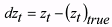
a one-day grid over a four-year interval from December 1, 1999, to November 30, 2003. Fig.
1 illustrates the time histories of the estimated correction parameters b1 and b2 for the
NRLMSIS-00 density model. Using these data, everyone can independently estimate the
corrections to the NRLMSIS-00 model density and take them into account in orbit
calculations by the formula
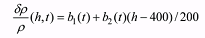 (1) (1)The effectiveness of this process was evaluated by comparing the orbit determination
and prediction results obtained without and with the constructed density corrections. The
application of density corrections for the NRLMSIS-00 model reduced the scattering of
ballistic coefficient estimates from 2 times for eccentric orbits up to 5.6 times – for near-
circular orbits. The reduced scattering in the ballistic coefficient values indicates that the
various complexities in the physics of the atmosphere are more consistently modeled with the
density corrections (Ref. 2).
In the current paper, the initial emphasis is on the basic statistical analysis of the
considered parameters (density correction parameters and solar activity and geomagnetic
index). The longer term goal is to develop relationships of the form:
 (2) (2)The following are provided:
Next the construction of the matrix autoregression equations for the parameters of
density correction and the application of these equations for forecasting the density correction
is considered.
Finally the application of the ARIMA model to analyze and forecast the time series of
density corrections is considered.
2. STATISTICAL PROPERTIES OF THE DENSITY CORRECTION TIME SERIES FOR THE NRLMSIS-00 MODELFigure 1 presents plots of the time histories of the b1 (‘blue’) and b2 (‘black’) coefficients for
the density corrections in the NRLMSIS-00 model. The data processing technology used to
generate the NRLMSIS-00 density corrections (Refs. 3 thru 6) is similar to that used
previously for the GOST density model. The only distinctions were:
In total, 1460 daily estimates of each of the b1 and b2 parameters were obtained.
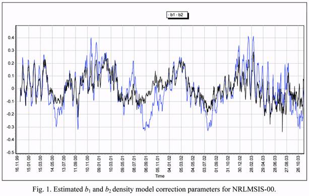
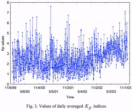
Figures 2 and 3 give the solar activity and geomagnetic index data for the time interval.
Further details regarding the construction of the density corrections for the NRLMSIS-00
density model are given in the authors’ previous paper, Ref. 1.
The natural approach to construction of mathematical models is based on obtaining,
accumulating, and analyzing data on the evolution of the object’s state in time when these
data are accessible to measurement. In this, we follow the overall approach of Box and
Jenkins (Ref. 9).
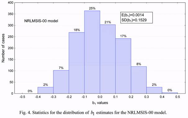
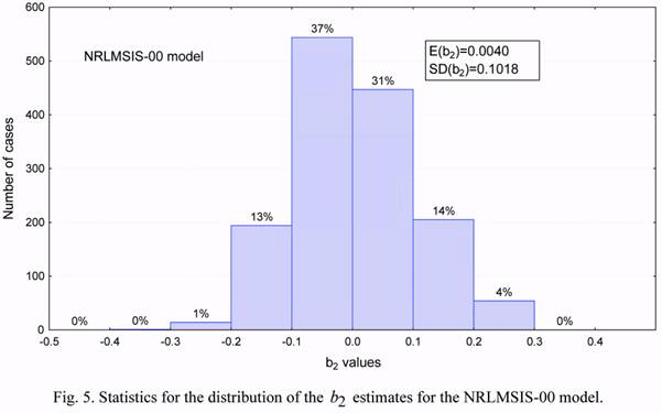
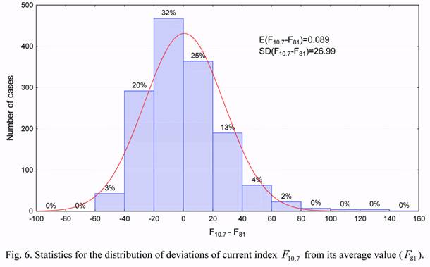
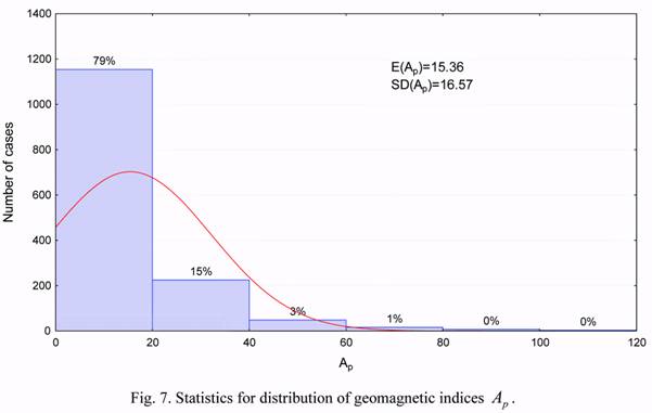
Figures 4 to 7 show the statistical distribution of the observed estimates of the b1 and b2
density correction coefficients, as well as the solar activity and the geomagnetic index. These
distributions, except for Figure 7 for the geomagnetic index, are close in their form to normal
distributions. This implies the possibility of applying both the statistical methods developed
for random values having normal distribution, and the linear relations between considered
parameters.
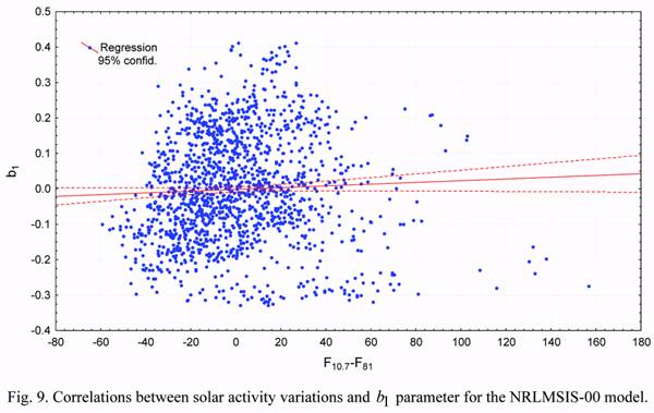
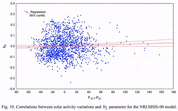
Figures 8 through 12 give scatterplots for various pairs of the considered parameters.
The least-squares regression line is also presented in each of these plots. It is seen from
Figure 8 that a significant correlation exists between the b1 and b2 parameters. The greater the positive value of the b1 coefficient, the stronger the increase of density correction with
altitude (b2). At the same time, it is seen from Figure 9, that the relation between the b1
values and the solar activity variations is weak. Similarly, Figure 10 shows that the relation
between b2 and the solar activity variations is weak. Figure 11 shows that the correlation of
the b1 values with the geomagnetic index variations is weak. Figure 12 shows that the
correlation of the b2 values with the geomagnetic index variations is also weak.
The previous data are characterized by the fact that they do not take into account the
time relations between the parameters. We now consider the relations between the analyzed
time series data, namely their auto correlation and cross-correlation functions. The
autocorrelation is the correlation of a series with itself lagged by a particular number of
observations. The auto correlation at lag k is (Ref. 9, p. 26):
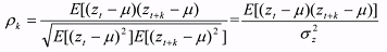 (3) (3)where
 and
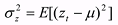 The auto correlation at zero lag is one.
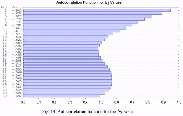
Figures 13 and 14 give the autocorrelation of the b1 and b2 series, respectively. The lag
values in these figures are plotted on the vertical axis for lags from one (1) to thirty (30) days.
A common feature of these functions is the presence of a local maximum in the area of lag
values of 25 to 29 days. This effect is a natural manifestation of the well-known monthly
cycle of solar activity influencing the state of the upper atmosphere.
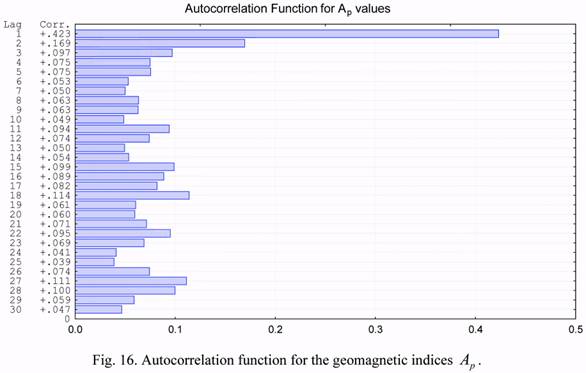
Figure 15 gives the autocorrelation of the difference between the daily value of the F10.7 solar activity and the 81 day average F81. Figure 16 gives the autocorrelation for the
geomagnetic indices Ap.
The b1 and b2 time series have very large values of autocorrelation coefficients for lags
less than 7 (seven) days. They exceed the value of 0.7. The corresponding values for the
solar activity and geomagnetic index are much lower. This circumstance suggests the
possibility of developing rather efficient algorithms for short-term forecasting of the b1 and b2
future values.
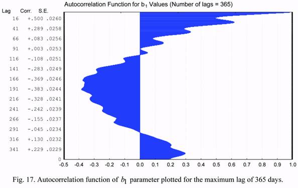
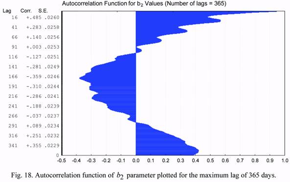
Figures 13 and 14 (b1 and b2 series) show plots of the autocorrelation functions for the
maximum lag of 30 days. Let us consider now similar plots constructed for the maximum lag
of 365 days. These plots are shown in Figures 17 and 18. The annual effects in the
corrections to atmospheric density, constructed for the NRLMSIS-00 model, are well seen in
these plots. The maximum values of semi-annual correlations the b1 and b2 parameters are
equal to -0.384 and -0.379, respectively. The values of the annual correlations for these
parameters are equal to 0.296 and 0.422. All these data indicate that the given model poorly
represents the monthly and annual changes of density in the upper atmosphere, and show
possible directions for its improvement.
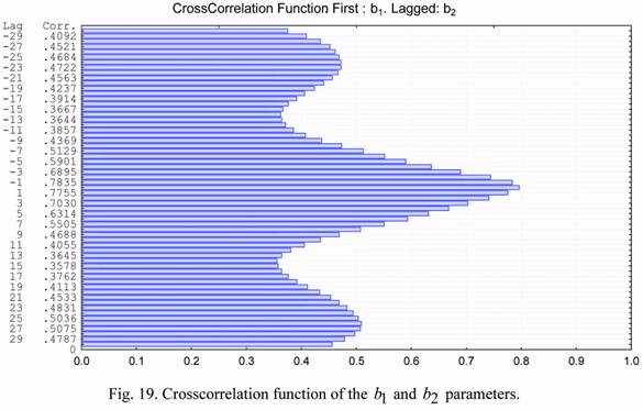
The data analysis tool employed for the identification of transfer function models is the
cross correlation function between the input and output (Ref. 9, Chap. 11). The cross
correlation function at lag k is given by
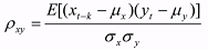 (4) (4)where μx and μy are the corresponding expected values for the two time series and σx and σy
are the respective standard deviations.
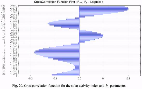
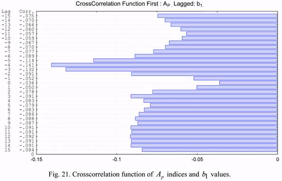
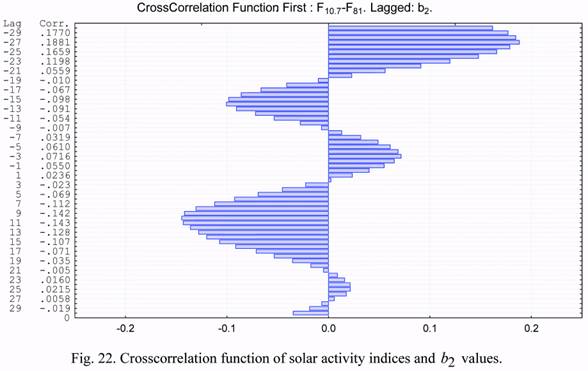
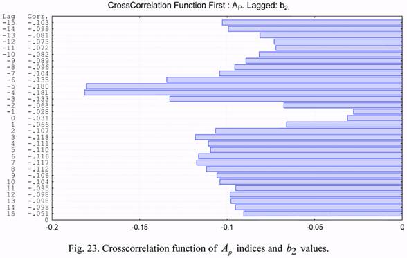
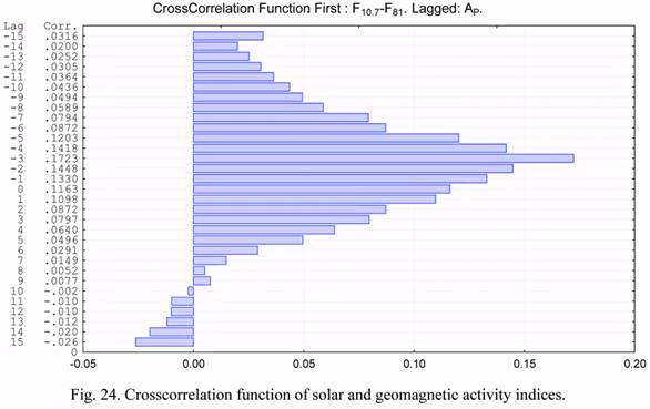
The cross correlation functions of the considered parameters are presented in Figures 19
through 24. Based on the presented cross correlation functions, one can draw conclusions on
the possibility of developing an algorithm for forecasting density correction coefficients for
the NRLMSIS-00 model using their previous values.
The cross correlations of the b1 and b2 time series are significant for the NRLMSIS-00 model. Values of the cross correlation coefficients exceeding 0.50 were revealed for the
NRLMSIS-00 model on lags of +/-9 days and on the monthly lag.
The cross correlations of the b1 and b2 series with solar activity were much smaller.
The cross correlations of the b1 and b2 series with the geomagnetic index are also much
smaller.
Similar statistical data for the GOST atmosphere density model (Ref. 10) also have been
obtained. These results are given in Ref. 11.
Overall, the given results for NRLMSIS-00 suggest the urgency of application of time
series analysis techniques for identifying the nature of the phenomena represented by the time
series of density correction estimates and for their forecasting (the prediction of future values
of the b1 and b2 time series).
3. THE USE OF AUTOREGRESSION EQUATIONS FOR FORECASTING THE DENSITY CORRECTION PARAMETERSThe technique for constructing the autoregression equations for vectorial processes was
presented in Section 3.4 of Ref. 12 and in Ref. 13. The intent is that using this technique will
make it possible to reveal the time regularity of the considered parameters, which will allow
for more efficiently predicting the parameters as compared to the case of using simplified
methods. In the case, where the state of some object (in our case - the atmosphere) at any
time instant is characterized by some vector, and the time series describing the change in the
state vector are stationary, the mathematical model of the objects can be represented as a
vector autoregression process of the type
 (5) (5)Here: a) zt is the n-dimensional vector, b) Фp,j, j=1, …, p are the n-dimensional matrix coefficients of the autoregression process, and c) ut is the vector of a random variable.
As the state vector components we shall consider the values of the b1 and b2
parameters of density corrections, as well as the values of solar and geomagnetic activity
indices (F7.10 and Kp). Thus, in our case the state vector zt is 4-dimensional one. Its values are known on the same time interval with the step of 1 day. They are presented in Figures 1
through 3 of this paper. Below, in analyzing solar activity, we shall consider the difference of
the current F7.10 index value and the 81-day running average centered on the day of interest
(F81).
As the initial data for forecasting we have used the set of values of density correction
parameters b1 and b2, as well as the values of solar and geomagnetic activity indices
presented in Figures 1 through 3. The statistical characteristics of state vector components are
presented in Table 1.
Table 1. Statistical characteristics of state vector components
The values of autoregression matrix factors of the second order, Ф1,2 and Ф2,2, were presented in Ref. 11. The formulas are:
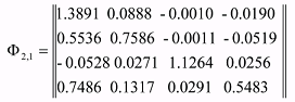 (6) (6)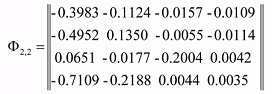 (7) (7)We note that the matrices given in Equations (6) and (7) are specific to the specific four
year interval and the choice of the NRLMSIS-00 density and the specific parameterization of
the solar activity and geomagnetic index data.
The standard method for determining the matrix coefficients Фp,j is based on the
construction and solution of the so-called Yule-Walker equations (Ref. 9). The solution of the
Yule-Walker equations in the explicit form (see Equation 3.2.7 in Ref. 9) is not always
convenient because of difficulties associated with the matrix inversion of high dimension.
More convenient is the recurrent solution procedure, which allows one to obtain the solution
at the (p+1)th step using the results of the pth step. Such a procedure is developed for vector
processes and described in Ref. 13.
The forecasting is carried out, based on the model given in Equation (8).
 (8) (8)Forecasting was carried out using Equation (8) according to two distinct test protocols:
The normalized forecasting errors were calculated for each predicted point using the
following equation:
 (9) (9)The mean values and the standard deviations of the normalized forecasting errors were
calculated based on the accumulated values of the normalized forecasting errors.
Comment. The first version of forecasts relates to the conditions of applying the current
known estimates of b1 and b2 parameters of density correction, as well as of solar and
geomagnetic activity indices for short-term forecasting of atmospheric density. Such
calculations characterize the efficiency of application of density corrections for solving the
operative ballistic tasks. The second version of forecasts allows for estimating the possibility
of application of the autoregression equations (8) under the conditions of absence of current
estimates of b1 and b2 parameters of density corrections. It is based on using the current
estimates of solar and geomagnetic activity indices only. The results of such calculations
characterize the possibility of application of the autoregression equation (8) as an addition to
the atmosphere model. They are based only on using the found dependences of b1 and b2
parameters on solar and geomagnetic activity variations.
Table 2. Statistical characteristics of normalized errors
For the first version of the test protocol, the basic forecasting results (the statistical
characteristics of normalized errors) are presented in Table 2 and in Figure 25. It is seen from
these data that for forecasting intervals up to 4 days the SD of normalized errors of b1 and b2
parameters change nearly linearly in the range of values from (0.2-0.3) to (0.5-0.6). The errors in the forecasting of the solar activity are slightly greater. For the geomagnetic index,
the corresponding characteristics vary from 0.80 to 1.0. It is natural that, later on, as the
forecasting interval increases, the SD of normalized errors of all parameters tends to the value
of 1.0. The average values of normalized errors in all cases are much lower, than the standard
deviations.
Thus, the presented results testify to a rather high efficiency of the application of the
vectorial autoregression equations for short-term (up to 4 days) forecasting of density
corrections. As compared to forecasting without density correction (SD(…)=1.0), the errors
of calculations of b1 and b2 parameters decrease 2-5 times for the forecasting interval of 1
day and 2 times – for the forecasting interval of 2 days. For forecasting intervals of 10 days,
the application of the autoregression equations results in about 15% decrease in the errors as
compared to calculation versions without density corrections.
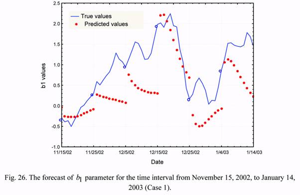
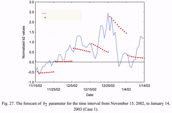
Figures 26 and 27 show examples of forecasting the b1 and b2 parameters and their
comparison with accurate (known) values. The data of these figures demonstrate the
possibilities of application of the autoregression equations for forecasting these time series.
The account taken of previous values of the state vector (in this case - for two time instants)
and general (averaged) statistical laws does not allow the prediction of the random (not
regular) variations of parameters.
In carrying out calculations by the second version of the test protocol, the forecasting
results for the first 100 steps after starting were not included in the statistical error data,
Equation (9). The statistical characteristics of the normalized errors (the average values and
standard deviations) were determined on the basis of forecasting results related to the time
interval beginning 110 days after starting (1350 realizations).
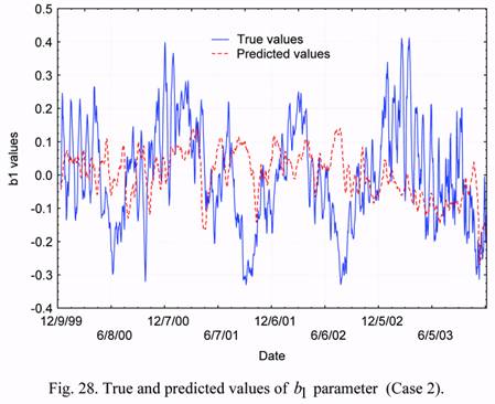
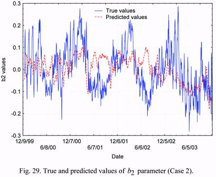
Figures 28 and 29 show the results of forecasting both the b1 and b2 parameters and comparison of the forecasts with the corresponding true data. One can see from the presented
results that, on the average, the forecasted values of parameters are lower than the observed
variations. Besides, in some cases, essential divergences between their general behaviors are
observed. In particular, in June-August of years 2001 and 2002 the forecasted values of
parameter b2 are positive, whereas the observed (true) values are negative. However, such a
divergence is absent in the data for year 2003: rather good agreement is observed in this case.
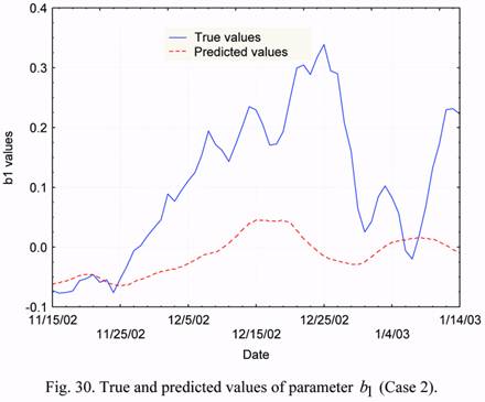
As an example, for the time interval from November 15, 2002, to January 14, 2003, the
corresponding results are presented in Figures 30 and 31 in a larger scale. These data show
once again, that the forecasting of b1 and b2 parameters without taking into account their
current estimates (i. e. based on the data on solar and geomagnetic activity only) does not
allow one to obtain an acceptable agreement between the predicted and true values. Table 3
shows the summary statistical characteristics of forecasting results.
For correct interpretation of the Table 3 data one should remember that the estimates of
b1 and b2 parameters were determined by means of long-term forecasting, whose results
depend on the current values of solar and geomagnetic activity only. The forecasting of
F7.10 and Kp parameters was carried out for one step (1 day) only. After this, the true values
were used as the initial data for forecasting. So, the statistical characteristics for these
parameters were obtained by forecasting for 1 day.
Table 3. Statistical characteristics of normalized errors (Case 2)
The following conclusions arise from the results of the second version of calculations:
4. APPLICATION OF THE ARIMA MODEL TO ANALYZE AND FORECAST THE TIME SERIES OF DENSITY CORRECTIONSThe task we consider in this section is formulated as follows: to construct simple scalar
models describing the b1 and b2 time series of density corrections for the NRLMSIS-00
model, to smooth them and to predict the future values of the time series using observations
up to the current time instant. Unlike the previous section, where the autoregression model
was used, we now use the ARIMA methodology for the solution of this task. The ARIMA
model describes the consecutive elements of the series in terms of specific, time-lagged
(previous) elements (the Autoregression hereafter) and a linear combination of moving
average values for this time series (the Moving Average hereafter). The ARIMA
methodology was developed by Box and Jenkins (Ref. 9). It has gained enormous popularity
in many areas and research practice, which confirms its power and flexibility. However,
because of its power and flexibility, the ARIMA is a complex technique; so, it is not easy to
use it: this requires a great deal of experience, although it often produces satisfactory results.
The latter depends on the researcher's level of expertise.
The general model introduced by Box and Jenkins includes autoregressive as well as
moving average parameters, and explicitly includes differencing in the formulation of the
model. Specifically, the three types of parameters in the model are: the autoregressive
parameters (p), the number of differencing passes (d), and moving average parameters (q). In
the notation introduced by Box and Jenkins, the models are summarized as ARIMA(p,d,q).
For example, a model described as ARIMA(0,1,2) means that it contains 0 (zero)
autoregressive (p) parameters and 2 moving average (q) parameters, which were computed for
the series after it was differenced once.
Thus, we have to decide, how many (p,d,q) parameters of the ARIMA model are
necessary to describe adequately the behavior of observed b1 and b2 time series for the density
corrections to the NRLMSIS-00 model. The determination of these parameters for the
ARIMA model is based on analysis of the statistical characteristics of the b1 and b2 time series. In particular, the input series for ARIMA needs to be stationary; that is, it should have
a constant mean, variance, and autocorrelation through time. Therefore, usually the series
first needs to be differenced until it becomes stationary. The number of times the series needs
to be differenced to achieve stationarity is reflected in the d parameter. In order to determine
the necessary level of differencing, one should examine the plot of the data and the
autocorrelogram. Significant changes in the level usually require first-order non-seasonal
(lag=1) differencing; the strong changes of a slope usually require second-order non- seasonal
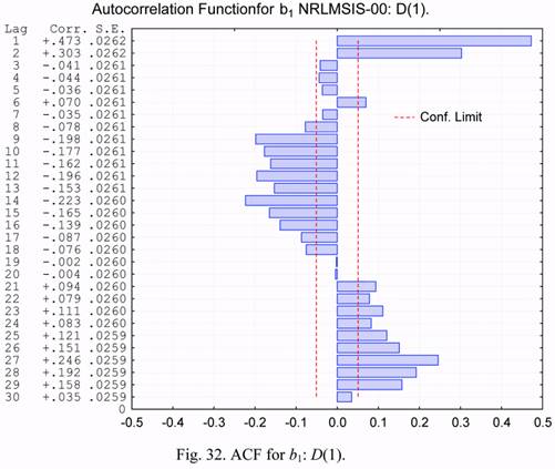
differencing. It is seen from the plots in Figures 13 and 14 that the estimated autocorrelation
coefficients for b1 and b2 decline slowly at longer lags. In the ARIMA model first-order
differencing is usually required in this case. However, one should keep in mind that some
time series may require either little or no differencing, and that over differenced series may
produce less stable coefficient estimates. Therefore, we shall try to construct the model with
first-order differencing.
At the model identification phase we also need to decide, how many autoregressive (p) and moving average (q) parameters are necessary to yield an effective but still parsimonious
model of the process. “Parsimonious” means that it has the fewest parameters and greatest
number of degrees of freedom among all models that fit the data. Major tools used in the
identification phase are plots of the series, the correlograms of the autocorrelation function
(ACF), and the partial autocorrelation function (PACF). The decision is not straightforward,
and in less typical cases it requires not only experience but also a good deal of
experimentation with alternative models. However, the majority of empirical time series
patterns can be satisfactorily approximated using one of the 5 basic models that can be
identified based on the shape of the autocorrelogram (ACF) and the partial autocorrelogram
(PACF). The following brief summary is based on practical recommendations by Pankratz
(Ref. 14).
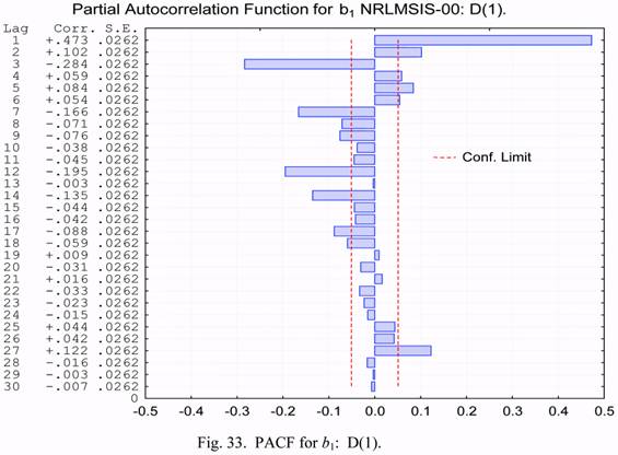
The PACF plot for the same time series is shown in Figure 33. It is seen from this plot,
that spikes are observed for various lag values. Therefore, none of models mentioned above
is suitable for describing the statistical characteristics of the b1 parameter.
For the initial analysis we choose the model, which can be described as ARIMA(2,1,0)
in the ARIMA notation, i.e. p=2, d=1, q=0. For b1 the following estimates and their standard
errors for the ARIMA (2,1,0) model parameters were obtained: p(1)=0.42443 (SD=0.02608),
p(2)=0.10209 (SD=0.02608). The initial and final sums of squares (SS) are equal to 1.3379
and 1.0282, respectively. The number of observations used to estimate the model parameters
was equal to 1458.
All-round analysis of the residuals is necessary for estimating the quality of the
constructed model. The qualitative model should have the independent residuals containing a
noise without systematic components. In particular, the ACF of residuals should not contain
any periodicity.
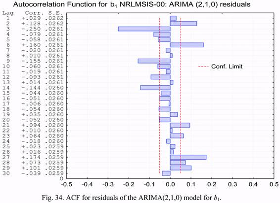
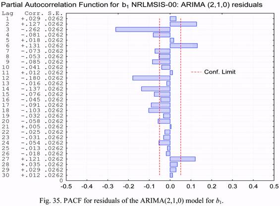
In Figures 34 and 35, plots of the autocorrelation and partial autocorrelation functions
for the residuals corresponding to the ARIMA(2,1,0) model are presented. It is seen from
these plots, that the correlation score of the residuals exceeds the confidence level. This
means that the model we have chosen describes the observed process inadequately.
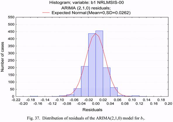
For completeness, Figure 36 gives the plot of residuals vs. time, and Figure 37 shows
the histogram of residuals distribution. In particular, it is seen from the plot in Figure 36, that
a heightened level of residuals was observed in 2003.
Thus, the simple ARIMA(2,1,0) model we have constructed does not adequately
describe the observed time series for b1. Let's try to find an alternative model for these data.
For this purpose we shall adjust successively the p and q input parameters of the ARIMA
model for the fixed value of parameter d=1. For each set of input parameters we shall
estimate the model’s parameters using the function minimization procedures. In practice, this
requires calculations of the sums of squares (SS) of the residuals because the estimation
procedure minimizes the sum of squares of residuals for the model. Therefore, we shall
choose the ratio of the final SS value to the initial one as a main criterion for comparison of
constructed models for various p and q. The initial SS values are the same for all comparing
models. Therefore the lower the value of this quantity, the better is the constructed model.
However, it is necessary to have in view in this case, that the qualitative model should be
economical and have independent residuals containing only the noise without systematic
components.
Table 4 gives the ratios of final SS values to initial ones for various ARIMA(p,1,q)
models, which were constructed for the b1 and b2 time series. On the basis of analysis of the
presented data and guided by the necessity of selecting an economical model, the
ARIMA(6,1,6) model was chosen both for b1 and b2 series.
Table 4. The ratios of final SS values to initial one for various ARIMA(p,1,q) models
Table 5 contains the estimates of p(j), q(j) (j=1,2 … 6) parameters for the
ARIMA(6,1,6) model, their standard errors (SD) and the t-values (parameter estimates
divided by standard errors). These characteristics are given both for b1 and b2 time series. It
follows from the presented data, that all obtained estimates of parameters are significant.
Table 5. Parameter estimates for the ARIMA(6,1,6) model for b1 and b2 time series
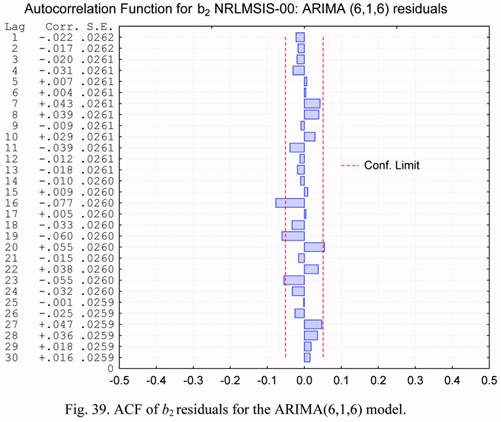
Figures 38 and 39 show the ACF plots of residuals corresponding to the case of using
the ARIMA(6,1,6) models to describe the b1 and b2 time series. One can notice from the
comparison of these plots with those in Figure 34, that the use of the more complicated
ARIMA(6,1,6) model has resulted in much less uncorrelated residuals. This means that the
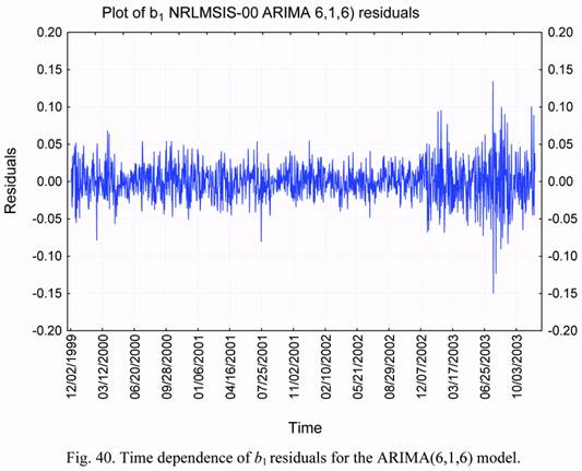
chosen ARIMA(6,1,6) model describes the observed time series more adequately. Figure 40
shows the time dependence of b1 residuals for the ARIMA(6,1,6) model. It is seen that,
visually, the plot in this figure only slightly differs from the plot for the ARIMA(2,1,0) model
presented in Figure 36. The heightened level of residuals since the end of 2002 is noticeable
for both models. As to comparison of the dispersion characteristics of residuals for these
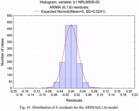
models, the distribution histogram for b1 residuals, corresponding to the ARIMA(6,1,6)
model, is presented in Figure 41. The normal distribution curve is superimposed in the same
figure. One can conclude from the comparison of the data of distributions in Figures 41 and
37, that the application of the ARIMA(6,1,6) model has led to a reduction in the spread of
residuals by 9% approximately, i. e. from 0.0262 down to 0.0241. The ratio of the SD of the
residuals for the ARIMA(6,1,6) model to the SD of the b1 time series (which is equal to
0.1529, see Figure 4) equals about 16%.
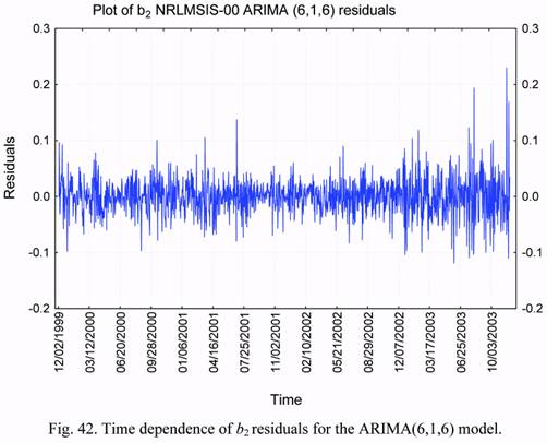
Figure 42 plots the time dependence for the b2 residuals corresponding to the use of the
ARIMA(6,1,6) model. It is also seen here that the residuals at the end of 2002 and in 2003
are larger than in 2000-2001 years. Apparently, this is due to the influence of the disturbing
factors on the estimates of the b1 and b2 values at the end of the analyzed interval. Probably,
the ARIMA model would be even more accurate in the absence of these factors. The
determination of the nature of mentioned factors requires additional investigations.
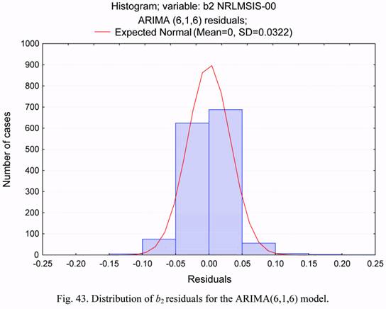
The histogram of distribution of residuals for b2 series is plotted in Figure 43. It is seen
that this distribution is unbiased. The SD of residuals equals 0.0322. Thus, with respect to
the SD of b2 time series (which is equal to 0.1018, see Figure 5), the SD of residuals for the
ARIMA(6,1,6) model equals about 32%. This value twice exceeds the ratio for b1 parameter,
thus testifying to a lower adequacy of the constructed model for b2 as compared to the model
for b1.
Now, when the models are constructed and their adequacy is estimated, it is possible to
estimate the quality of the forecasts constructed using these models. The time series of the
density corrections for the NRLMSIS-00 model was used as input data for forecasting. One
hundred and forty (140) versions of input data were chosen. The initial epoch of each forecast
is 10 days later than the previous one. The first forecast starts on January 19, 2000 (the 50th
day of considered four-year time period). Each forecast was executed over the interval from
one to 10 days.
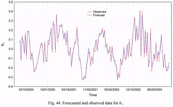
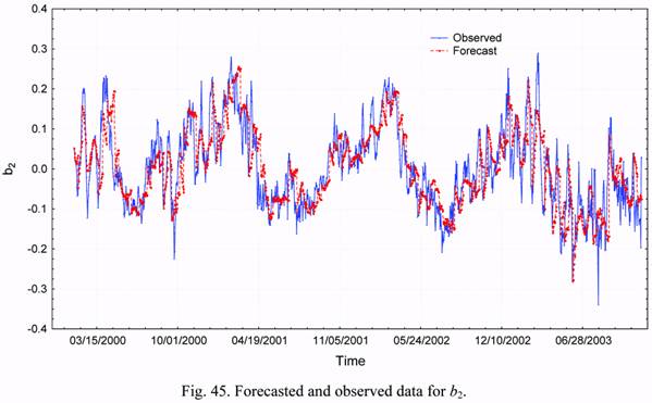
Figures 44 and 45 give the observed and forecasted values of the b1 and b2 parameters.
One can see that the forecasts for the b1 values are slightly more accurate than those for b2.
The errors in the b1 and b2 forecasts were calculated for each forecast point. Their
statistical characteristics, mean values and SDs of errors were calculated based on
accumulated estimates with the one-day step forecasting interval. The results of these
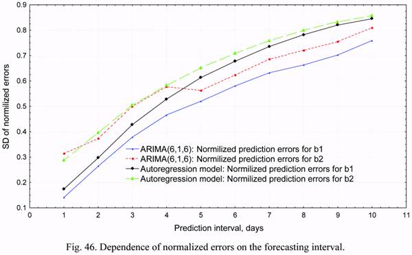
calculations (SD of absolute and normalized errors) of forecasting errors are given in Table 6
and in Figure 46. The dependences of prediction errors for b1 and b2 on the forecasting
interval, obtained by the autoregression model described in the previous Section, are also
plotted in Figure 46.
It is seen from these data that for forecasting intervals up to 4 days, the SDs of
normalized errors of the b2 parameter are identical for the ARIMA(6,1,6) and autoregression
models. For the b1 parameter, the ARIMA(6,1,6) model gives a little bit better results, than
the autoregression model. The ARIMA(6,1,6) forecasts are better than those of the
autoregression model at larger intervals both for b1, and b2. As a whole, the accuracy
behavior of these models depends on the forecasting interval. Some distinction in the
behavior of SD for normalized errors for b2 in the ARIMA(6,1,6) model can be explained by
insufficient number of forecasting statistics.
It is seen from the given data that on forecasting intervals up to 5 days the SD of
normalized forecasting errors for density correction parameters increase in the range of values
from 0.10 to 0.5. Further, as the forecasting interval increases, the SD of normalized errors
continues to be incremented and reach the values of 0.76-0.81 on the 10-day interval. Taking
into account the level of errors in estimating b1 and b2 values and the results of previous
investigations on the influence of density corrections to the LEO satellite prediction accuracy
(Ref. 15), one can assume that, at least on the intervals of about several days, the application
of constructed ARIMA models can give noticeable effect in increasing the accuracy of
solution of the problems related to LEO satellite tracking.
Thus, the obtained results testify to a rather high operational efficiency of the ARIMA
scalar models for short-term forecasting of density corrections. The accuracy of forecasting
with using these models exceed the accuracy of vectorial autoregression models by 5-10%.
Table 6. Forecasting error statistics
5. CONCLUSIONS
6. FUTURE WORKPossible directions of future activities are as follows:
Acknowledgement. The authors would like to acknowledge the representatives of the Space
Surveillance community in both the USA and in Russia for supporting the USA-Russia Space
Surveillance Workshops in 1994, 1996, 1998, 2000, 2003, and 2005. The specific contributions of Dr.
Ken Seidelmann (University of Virginia), Prof. Stanislav S. Veniaminov (Scientific Research Center
"Kosmos"), and Dr. Felix Hoots (General Research Corporation) in organizing these workshops are
noted. These workshops led directly to the collaboration reported in this paper. We are also grateful
to David A. Vallado (now at Analytical Graphics, Inc.), Dr. Chris Sabol (USAF/AFRL), Dr. Matthew
Wilkens (Naval Postgraduate School), and Mr. Zachary Folcik (MIT) for their continuing interest in
this work. We are very grateful to Dr. Thomas S. Kelso (Analytical Graphics, Inc.) for providing the
historical TLE sets using his personal WWW service. The Russian authors are grateful to Andrey
Bukreev (Head of the Space Informatics Analytical Systems) and Dr. Vladimir Agapov (Keldish
Institute of Applied Mathematics) for their current interest in this topic.
REFERENCES
LIST OF FIGURES
Размещен 4 декабря 2006.
| |||||||||||||||||||||||||||||||||||||||||||||||||||||||||||||||||||||||||||||||||||||||||||||||||||||||||||||||||||||||||||||||||||||||||||||||||||||||||||||||||||||||||||||||||||||||||||||||||||||||||||||||||||||||||||||||||||||||||||||||||||||||||||||||||||||||||||||||||||||||||||||||||||||||||||||||||||||||||||||||||||||||||||||||||||||||||||||||||||||||||||||||||||||||||||||||||||||||||||||||||||||||||||||||||||||||||||||||||||||||||||||||||||||||||||||||||||||||||||||||||||||||||||||||||||||||||||||||||||||||||||||||||||||||||||||||||||||||||||||||||||||||||||||||||||||||||||||||||||||||||||||||||||||||||||||||||||||||||||
|
|
|
|
|
|
|
|
