


|
|
|
|
|
|
|
|
REVIEW OF RESULTS ON ATMOSPHERIC DENSITY CORRECTIONS*Vasiliy S. YURASOV2, Andrey I. NAZARENKO3, Kyle T. ALFRIEND4, Paul J. CEFOLA52 Space Informatics Analytical Systems (KIA Systems), 20 Gjelsky per, Moscow, 105120, Russia
3 Space Observation Center, 84/32 Profsoyuznaya ul, Moscow, 117810, Russia
4 Texas A&M University, 701 H. R. Bright Building, Department of Aerospace Engineering, Texas A&M University, College Station, TX 77843-3141, USA
5 MIT Aeronautics & Astronautics Department, 59 Harness Lane, Sudbury, MA 01776, USA
1. INTRODUCTIONAtmospheric density mismodeling was, and remains, the dominant error source in the orbit
determination and motion prediction of LEO space objects. All known upper atmosphere
models describe with insufficient accuracy the real dynamic variations of density caused
mainly by the influence of solar and geomagnetic perturbations on the atmosphere.
One promising direction for increasing the accuracy of satellite orbit determination and
prediction for low Earth orbit satellites is the real-time estimation and application of density
corrections between the real density and the density calculated by the operational atmosphere model. This idea, offered at the beginning of the 1980s [1], is based on the usage of the
available atmospheric drag data on catalogued LEO satellites for construction of corrections
to the employed atmospheric density model. At any given time there are several hundred such
drag-perturbed space objects in orbit. The element sets for these space objects are updated as
an ordinary routine operation by the space surveillance systems (SSSs) a few times per day in
near-real time. Therefore, corrections to the modeled atmosphere density can be constructed
without significant additional costs.
The considered investigations are one of the examples of successful US-Russian
cooperative research projects in the area of space surveillance. The beginning of this long-
term cooperation was the Second US-Russian Space Surveillance Workshop held in Poznan,
Poland in July, 1996. Prof. A. I. Nazarenko presented there a survey paper on this topic [2]
and the interesting discussion of these problems took place with Dr. P. J. Cefola.
At the last few US-Russian workshops, discussions on atmospheric density problems
have become traditional. Our work on this topic has successfully continued during the two
years since the previous workshop at St-Petersburg. The most significant results of these years
are the following:
2. MATHEMATICAL STATEMENTThe estimation of un-modeled variations or the construction of atmospheric density
corrections using the available drag data for LEO space objects can be expressed in a general
form as a problem of functional minimization [6]
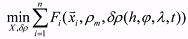 (1) (1)where n is the number of LEO SOs, chosen for the estimation of density corrections; xi
represents the ith SO state vector (i=1 thru n); X (x1, x2, ... xn ); Fi is the optimization criterion, applied to the ith SO for estimation of its motion parameters; ρm = ρm(h,φ,λ,t) is
the density calculated by the employed (base) atmosphere model (modeling density value); δρ(h,φ,λ,t) is the density correction function; h is altitude, φ is latitude, λ is longitude, t is time.
The knowledge of density corrections δρ(h,φ,λ,t) allows the calculation of the real values of the density at a point of interest in space
 (2) (2)To solve the minimization task (1) in the general case, the orbit determination process
and the density correction process should be considered as a single estimation process.
Searching for optimum estimations for the multi-parameter task (1) is a nontrivial problem.
Apparently, its correct solution is possible only in the presence of measurements meeting
certain requirements on precision, quantity, and spatial and temporary distribution. In our
approach, these processes are separated. In addition, due to the difficulty in observing the
functional relation of the density corrections to the latitude and longitude by using the
available satellite drag data, the density corrections were expressed only as a linear function
of altitude
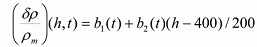 (3) (3)3. TECHNICAL APPROACH AND SOFTWAREWe have chosen the US SSS TLE data as a basic source of orbital information for the
construction of the atmospheric density corrections [7–12]. The choice of the TLE data is
explained, first, by their availability over the Internet, and, secondly, by the convenience of
obtaining both retrospective, and current TLE-orbits. Moreover, the current orbits are
accessible in a near-real time mode.
The satellite drag data, contained in the TLE-orbits, can not be directly used for
constructing the density corrections. For this reason, a special algorithmic approach and
software were developed for the automated data processing. The process of estimating the
density corrections based on the TLE data includes the following basic steps (see Fig. 1).
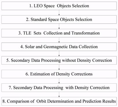 Fig. 1. Steps in the Construction and Test of the Density Corrections.
4. DENSITY CORRECTIONS FOR THE GOST AND NRLMSIS-00 MODELSThe described technique has been applied to two base atmosphere density models – GOST
and NRLMSIS-00 [9–11]. Time series for the b1 and b2 coefficients of the density corrections
model (3) for these models have been constructed on a one-day grid over the four-year
interval starting from December 1, 1999.
The corrections for the GOST model have been calculated using drag data on about 500
SOs. The daily number of estimates of the smoothed ballistic coefficients used for the
estimation of the b1 and b2 coefficients varies mainly from 400 up to 600. Almost 800, 000
estimates of the ballistic coefficients were used for the density corrections generated over the
four-year interval. Fig. 2 gives for the GOST model the time histories of the estimated b1 and b2 density model correction parameters defined in equation (3).
Due to the great volume of required calculations, only 16 carefully chosen SOs have
been used for construction of density corrections for the NRLMSIS-00 model. In 92% of the
NRLMSIS-00 cases, the daily number of ballistic coefficient estimates varies from 10 to 25.
The total number of ballistic coefficient estimates, obtained on these SOs for the four-year
time interval was 24,773. Fig. 3 illustrates the time histories of the estimated correction
parameters b1 and b2 for the NRLMSIS-00 density model.
Using the obtained data everyone can independently estimate the corrections to the
GOST or NRLMSIS-00 model and take them into account in calculations by formula (3).
As an example, the atmospheric density corrections to the NRLMSIS-00 model,
calculated for 2003, are given in Fig. 4 for altitudes of 200, 300, 400, 500 and 600 km. From
the presented plots it is visible, in particular, that the larger the height, the larger are the
differences between the real values of density and those calculated by the base model. So, the
maximum values of atmospheric density corrections for the NRLMSIS-00 density model
reached 25% at the 200-km altitude and 70% - at the 600-km altitude. Similar dependence of
the density corrections on altitude is observed also for the GOST model results.
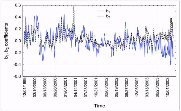 Fig. 2. Estimated b1 and b2 density model correction parameters for the GOST model.
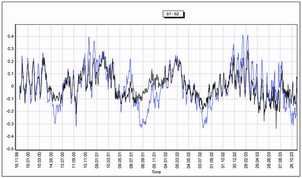 Fig. 3. Estimated b1 and b2 density model correction parameters for the NRLMSIS-00 model.
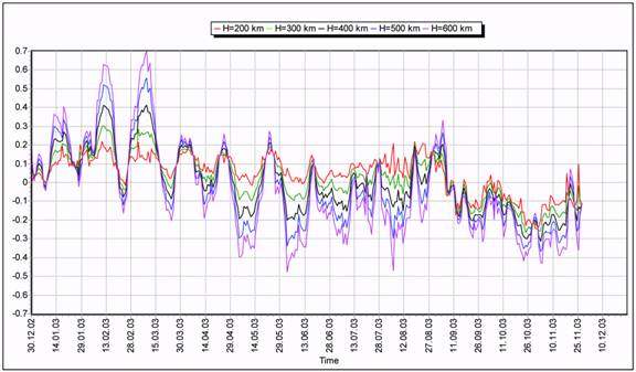 Fig. 4. Corrections to the NRLMSIS-00 model for 2003.
5. EVALUATION OF APPLYING THE DENSITY CORRECTIONSThe quality of the constructed density corrections to the base atmosphere model may be
evaluated by the comparison of the scatter of the orbit fitting ballistic coefficient estimates
obtained with and without the corrected densities. If the density corrections take into account
correctly the un-modeled density fluctuations, then the resulting ballistic coefficients for
spherical-shaped objects should have significantly smaller scatter. The results presented for
the Starshine 3 satellite in Fig. 5 confirm this regularity. Before the density correction the standard deviation (SD) of ballistic coefficient values was 12.8% for this satellite. After
applying the density correction, the standard deviation decreased down to 2.8%. For the
NRLMSIS-00 model such comparisons have been carried out for 25 SOs, of which 9 SOs
were not included in the list chosen for the density correction process. Fig. 6 presents the
scatterplot of ballistic coefficients estimates for all SOs, obtained without (Kb-variations) and
with (Kbf-variations) density corrections taken into account. The analysis of these data
indicates that the application of density corrections to the NRLMSIS-00 model has eliminated
the long-periodic variations in the ballistic coefficient estimates caused by the errors in the
atmospheric density model. On the average, the density corrections to the NRLMSIS-00
model reduced the scattering of the ballistic coefficient estimates by a factor of 3.6.
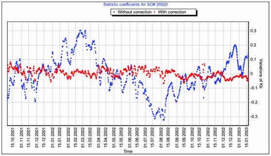 Fig. 5. Ballistic coefficient variations obtained for Starshine 3 satellite without and with density
correction (GOST)
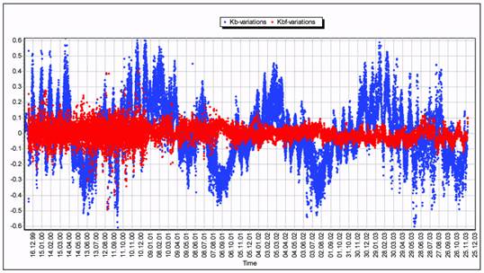 Fig. 6. Variations of ballistic coefficients before and after applying the density model correction (all
25 SOs) (NRLMSIS-00).
The comparative analysis of variations of ballistic coefficients obtained before and after
density corrections has been fulfilled for the GOST model also. The generalized statistical
characteristics of the distribution of variations for this model are presented in Table 1. The
comparison interval includes data over the entire four-year interval, from December 1999
through December 2003. The results of the data processing over this interval have shown that
the SD of ballistic coefficient variations, estimated for all SOs without atmospheric density
corrections, was equal to 23.4%. The number of estimates of the ballistic coefficients was
equal to 794,906. For the calibration SOs these values were equal to 15.8% and 97,881
respectively. The SD of ballistic coefficient variations, obtained with atmospheric density
corrections on 773,998 realizations, including all SOs, was equal to 14.4%. A similar
characteristic calculated for 96,475 estimates on the calibration SOs was equal to 8.7%. Thus,
the value of the scattering of the ballistic coefficient variations, calculated for all the SOs,
decreased 1.62 times when accounting for constructed atmospheric density variations, and
1.82 times for the calibration SOs.
The presented results support the conclusion that estimations of the upper atmosphere
density, obtained after density corrections, track the real changes of the density much better,
than the employed GOST and NRLMSIS-00 models.
Table 1. The generalized statistics for distribution of ballistic coefficient estimates
(the GOST model).
Let's now consider the influence of the atmospheric density corrections on the accuracy
of the orbit prediction. For the GOST model these results were obtained for two years of the
overall time interval: 2000 and 2002. The 2000 interval is of interest, because the upper
atmosphere was strongly perturbed during this period. The year 2002 was the quietest year
from the viewpoint of intensity and frequency of disturbances of the upper atmosphere
density. The orbit predictions were carried out for all the space objects that were chosen for
the experiment. To obtain the comparable error statistics across all satellites and for different
prediction intervals normalized error parameters were used [10]. Table 2 presents the
generalized statistical characteristics for the distribution of normalized prediction errors,
obtained with and without atmospheric density correction. The averaged values of the
standard deviation for the prediction errors, obtained without and with the corrections of the
atmospheric density, are equal to 29.2% and 16.5%, respectively, for 2000. For the calibration
SOs, the appropriate SD values are 27.9% and 13.7%. Thus, on the interval of 2000 the
density correction results in a reduction in the prediction errors of 1.77 times for all SOs, and
by 2.03 times for the calibration SOs. For the rather quiet period of 2002 the density
correction results in the accuracy increasing by 1.41 for all SOs, and by 1.78 for the
calibration SOs.
The influence of applying the density corrections on the accuracy of predictions for the
NRLMSIS-00 model has been estimated by comparison of the results of SO’s reentry time
predictions [12]. Table 3 generalizes data characterizing the influence of density corrections
to the NRLMSIS-00 model for Starshine satellites of spherical shape. It is seen from the data
of Table 3 that the application of density corrections to the NRLMSIS-00 model has decreased the prediction errors for satellites of Starshine series by factors of 5.7, 3.0 and 1.6.
The root-mean-square (RMS) values of reentry prediction errors were in the range from 4.9%
to 8.1% before density corrections. The residual level of RMS errors after density corrections
decreased to the range from 1.4% to 3.1%.
Table 2. The generalized statistics of prediction errors
Table 3. Statistics for reentry prediction errors for Starshine satellites.
Calculations, which demonstrate the impact of the density corrections on the reentry
prediction accuracy, were carried out additionally for 95 chosen LEO space objects having
arbitrary shapes. For the majority of the objects the prediction interval was limited to 10 days.
The average value of prediction numbers for SOs of this group was equal to 31. The average
value of RMS errors for the case of predictions without density corrections is equal to 9.1%.
The correspondent value of RMS after density correction equals 6.9%, i.e. it decreased by
32%.
6. ESTIMATION OF TRUE BALLISTIC COEFFICIENT VALUESFor calculating the density corrections for each ith space object, especially for calibration
satellites, it is necessary to know, as precisely as possible, the estimate of a ‘true’ value of the
SO’s ballistic coefficient we designated as ki. The ballistic coefficient is determined in our
calculations as
 (4) (4)where Cd is the dimensionless coefficient of drag, S is the cross-sectional area perpendicular to satellite’s motion, and m is the mass.
The estimate of the true value of a ballistic coefficient of our calculating was
determined as an average value of all the ballistic coefficient estimates for the given SO
 (5) (5)where kij denotes the jth ballistic coefficient estimate for the ith space object; n is the number of ballistic coefficient estimates obtained for the ith space object.
For verification, the true values of ballistic coefficients, estimated by us for the
NRLMSIS-00 model, have been compared with the similar estimates obtained in the
construction of the High Accuracy Satellite Drag Model (HASDM), and the theoretical values
calculated for spherical SOs [11]. Table 4 summarizes the results of the estimations of true
ballistic coefficient values that we have obtained for all 16 selected SOs. The first column
gives the NORAD catalog numbers for space objects. The second and third columns present,
respectively, the numbers of estimates (ni) and covering intervals, over which the estimates
of true values of ballistic coefficients were obtained using the NRLMSIS-00 model. The true
values of ballistic coefficient estimates (5) are presented in the fourth column. For
comparison, the estimates of true values of ballistic coefficients B/2, obtained in the
HASDM construction [16–19], are presented in the fifth column. These data were calculated
by averaging the ballistic coefficient estimates obtained over a 30-year interval for all
considered SOs, except the satellites of Starshine series. The Jaсchia atmosphere model [20]
has been used as the base model in the HASDM. The sixth column contains the theoretical
values of the ballistic coefficients for some SOs of spherical shape calculated by formula (4).
The seventh column of the table presents the relative differences, in percentage, between our
estimates of true values of ballistic coefficients and estimates obtained during the HASDM
construction. And the last column gives the relative differences, in percentage, between our
estimates of true values of ballistic coefficients and theoretical estimates.
The data of Table 4 testify to a very good coincidence of our estimates of true ballistic coefficient values with the estimates obtained during the HASDM construction. A difference
between these estimates equals only 1.3% on the average! The maximum distinction between
these estimates obtained by data averaging over different time intervals and for different
atmosphere models is equal to 4.3%.
It follows from the analysis of the last column data, that our estimates agree a little
worse with the theoretical estimates of ballistic coefficients, which were calculated under an
assumption that the aerodynamic drag coefficient Cd is equal to 2.1 for all SOs. The
maximum distinction of obtained estimates of true values of ballistic coefficients from their
theoretical values equals -6.8%. The average value of difference between experimental and
calculated values equals -3.39%. It is also seen from these data that for the majority of SOs,
the theoretical value of the ballistic coefficient is greater than the experimental one. Note also
that we have calculated the theoretical values for Cd=2.1, though in reality it is recommended
to let Cd=2.2 for spherical-shaped SOs. Taking these circumstances into account, one can
suppose that the NRLMSIS-00 atmosphere model has a bias on the considered time interval.
As a result, this model may give at 200-600 km altitudes more high values of density, on the
average. The relative value of this bias can lie in the range from 3% to 8%, and, possibly, this
value depends on the altitude.
Table 4. True ballistic coefficients.
7. COMPARISON OF THE GOST AND NRLMSIS-00 RESULTSThe corrections to density that we calculate from the drag data of LEO space objects are, in their essence, the errors in the used models. By this reason it is interesting to compare the
statistical characteristics of these corrections obtained for various models. The results of this
comparison can be useful, for example, in selecting the atmosphere model for our
applications, when we have to decide, which model is better for solving some specific task.
These results can also be used for estimating the a priori errors of prediction.
We obtained the density corrections for two atmosphere models, namely, the GOST and
NRLMSIS-00 models, over the four-year interval. Table 5 presents the statistical
characteristics (the mean values and standard deviations) of density corrections for each of
these two models. These characteristics were calculated for altitudes of 200, 300, 400, 500
and 600 km. Fig. 7 gives the plots of the time history of density corrections for the 600 km
altitude. Fig. 8 shows the linear regression line fitted to the errors of the GOST model as a
function of altitude. In the same figure the 95% confidence interval for the regression line is
plotted as well. Similar scatterplots are presented in Fig. 9 for the NRLMSIS-00 model. The
analysis of these data allows one to draw the following conclusions:
Table 5. True ballistic coefficients.
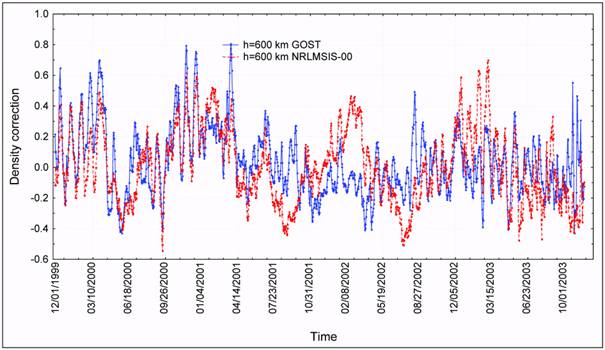 Fig. 7. Comparison of density corrections constructed to the GOST and NRLMSIS-00 models for
600 km altitude.
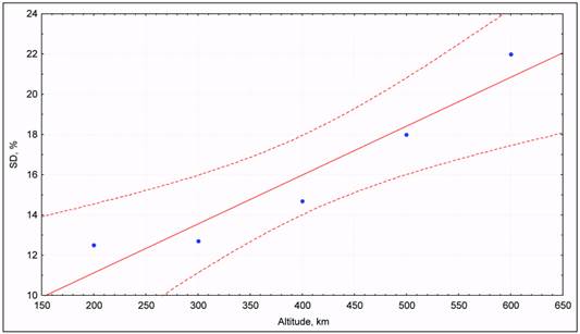 Fig. 8. Altitude linear regression for errors of GOST model.
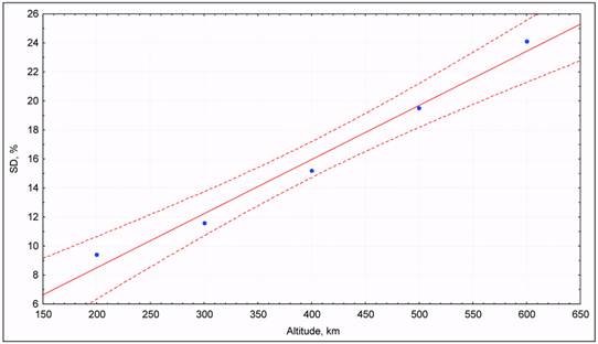 Fig. 9. Altitude linear regression for errors of NRLMSIS-00 model.
8. INDIVIDUAL SO’s FEATURESSometimes accounting for the density corrections does not increase the orbit prediction
accuracy. This can be due to the individual SO’s features of aerodynamic characteristics. Such
features can be caused, for example, by the long term character of the SO’s attitude motion.
Variations of a ballistic coefficient value, in some cases, for such a SO can become a main
reason for motion prediction errors in the upper atmosphere.
Analysis has shown that the detection such SOs is possible by comparison of their
ballistic coefficients variations, obtained without and with density corrections. The
application of density corrections to the model does not eliminate the long-periodic variations
in the ballistic coefficient estimates for such SOs. The common regularity in ballistic
coefficient variations of these SOs is their prominent periodicity with high amplitude, whose value is commensurable with the mean value of ballistic coefficient estimates. Fig. 10 shows
the plots for estimates of the ballistic coefficient, obtained with and without atmospheric
density corrections, for SO #26124. For this SO the maximum estimates for ballistic
coefficient differ 5.0 times from minimum ones, both before and after density corrections, and
ballistic coefficient variations have a period of about 5.6 months.
The individual features in the aerodynamic characteristics behavior of SOs can be
revealed by the analysis of their history of ballistic coefficients estimates obtained with
density corrections. Further, these regularities can be used for forecasting the SO’s ballistic
coefficient variations and their accounting in the SO’s motion prediction. The obtained results
in this area [12] show that perspective methods for the solution of this task can be an auto
regression and ARIMA time series analysis and forecasting methods [21–23].
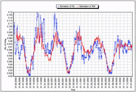 Fig. 10. Ballistic coefficient variations obtained for SO#26124 without and with density corrections.
9. CONCLUSIONSThe primary source of errors in orbit determination and prediction for the LEO space objects is the inaccuracy of the upper atmosphere density models. The existing models do not
represent the actual density variations with an acceptable accuracy. An effective approach for
monitoring the current atmospheric density variations is based on using the available SSS
drag data for the LEO space objects. This approach was first conceived more than 20 years
ago and has been gradually improved since then. For the last few years our studies in this
direction have been connected with the practical application of techniques, and have
developed software for the construction of atmosphere density corrections using the TLE sets
as input observational data. As a result, the density corrections for the GOST and NRLMSIS-
00 models were constructed with a one-day grid over a four-year interval starting in
December 1999. The effectiveness of this density correction process was evaluated by
comparison of the orbit determination and prediction results, obtained with and without taking
into account the estimated density variations. A preliminary comparison of the obtained data
with the HASDM results was made.
The applied technique and obtained results can be useful for the solution of a number of
practical tasks, including:
The obtained results testify to the efficiency of the applied technique and the necessity
of the continuation of work on monitoring the un-modeled variations in the atmosphere
density. In this connection, the actual directions of the further work are suggested as follows:
Acknowledgements. The authors would like to acknowledge the representatives of the Space
Surveillance community in both the USA and in Russia for supporting the US-Russian Space
Surveillance Workshops in 1994, 1996, 1998, 2000, 2003 and 2005. The specific contributions of Dr.
Ken Seidelmann (now at the University of Virginia), Dr. Stanislav S. Veniaminov (Scientific Research
Center "Kosmos"), Dr. Felix Hoots (General Research Corporation), Dr. Alexander V. Stepanov, and
Dr. Alla S. Sochilina (both from Central Astronomical Observatory at Pulkovo of the Russian
Academy of Sciences) in organizing these workshops are noted. These workshops led directly to the
collaboration reported in this paper. The authors would also like to acknowledge their co-workers at
the MIT Lincoln Laboratory and at the Charles Stark Draper Laboratory. We are also grateful to
David A. Vallado (now at Analytical Graphics, Inc.) and Dr. Chris Sabol (USAF/AFRL) for their
continuing interest in this work. We are very grateful to Dr. Thomas S. Kelso (now at Analytical
Graphics, Inc.) for providing the historical TLE sets using his personal WWW service [14]. The
Russian authors are grateful to Andrey Bukreev (Head of the Space Informatics Analytical Systems)
for his current interest in this topic.
REFERENCES
Размещен 2 декабря 2006.
| ||||||||||||||||||||||||||||||||||||||||||||||||||||||||||||||||||||||||||||||||||||||||||||||||||||||||||||||||||||||||||||||||||||||||||||||||||||||||||||||||||||||||||||||||||||||||||||||||||||||||||||||||||||||||||||||||||||||||||||||||||||||||
|
|
|
|
|
|
|
|
 (6)
(6) (7)
(7)