


|
|
|
|
|
|
|
|
THE SEMIANNUAL THERMOSPHERIC DENSITY VARIATION FROM 1970 TO 2002 BETWEEN 200-1100 KMBruce R. BowmanAir Force Space Command, e-mail: bruce.bowman@peterson.af.mil
INTRODUCTIONThe semiannual density variation was first discovered in 19611. Paetzold and Zschorner
observed a global density variation from analysis of satellite drag data, which showed a 6-
month periodicity maximum occurring in April and October, and minimum occurring in
January and July. Many authors, such as King-Hele2, Cook3, and Jacchia4, analyzed the
semiannual effect from satellite drag during the 1960s and early 1970s. They found that the
semiannual variation was a worldwide effect with the times of the yearly maximum and
minimum occurring independent of height. However, the semiannual period was found to be
only approximate, as the times of occurrence of the minimums and maximums seemed to vary
from year to year. Generally the October maximum exceeded that in April and the July
minimum was deeper than that in January. None of the results showed any correlation of the
semiannual variations with solar activity. Thus, the main driving mechanism for the observed
variability in the semiannual variation remained a mystery. Jacchia4 first modeled the effect
as a temperature variation. However, he soon discovered difficulties with the temperature
model, and eventually modeled the semiannual variation as a density variation5,6. He also
found that the amplitude of the semiannual density variation was strongly height-dependent
and variable from year to year. However, he again found no correlation of the variation with
solar activity. All the previous analyses were limited to a relatively short time interval of a few years. More recent studies7,8,9 have combined together several years of satellite drag data
to analyze the semiannual variation, thus again missing the year-to-year variability. The
purpose of this current study is to quantify the year-to-year variation over the last three solar
cycles, and to prove or disprove the conclusion that the semiannual effect is not dependent
upon solar activity.
DATA REDUCTIONDaily temperature corrections to the US Air Force High Accuracy Satellite Drag Model’s
(HASDM)10,11 modified Jacchia6 1970 atmospheric model have been obtained on 13 satellites
throughout the period 1970 through 2002. Approximately 120,000 daily temperature values
were obtained using a special energy dissipation rate (EDR) method12, where radar and
optical observations are fit with special orbit perturbations. For each satellite tracked from
1970 through 2000 approximately 100,000 radar and optical observations were available for
special perturbation orbit fitting. A differential orbit correction program was used to fit the
observations to obtain the standard 6 Keplerian elements plus the ballistic coefficient. “True”
ballistic coefficients13 were then used with the observed daily temperature corrections to
obtain daily density values for different reference heights (average perigee heights). The
daily density computation was validated3 by comparing historical daily density values
computed for the last 30 years for over 30 satellites. The accuracy of the density values was
determined from comparisons of geographically overlapping perigee location data, with over
8500 pairs of density values used in the comparisons. The density errors were found to be
less than 4% overall, with errors on the order of 2% for values covering the latest solar
maximum. The latter decrease in error is largely due to increased observation rates.
Table 1 lists all the satellites used for this study. A variety of orbit inclinations, from
low to high, were used. The satellites with perigee heights below 600 km are in moderate
eccentric orbits with apogee heights varying from 1500 km to over 5000 km. The majority of
the satellites are spheres, which avoids the possibility of frontal area problems producing
invalid drag results.
Table 1. Satellites used for the semiannual density variation study.
Table is sorted by perigee height (in bold).
The semiannual variations were computed first by differencing the computed daily
density values with density values obtained from the HASDM modified Jacchia atmospheric model without applying both the daily temperature corrections and Jacchia’s semiannual
equations. If Jacchia’s model were perfect then the resulting differences would only contain
the observed semiannual variation. This is equivalent to computing the “Density Index” D
that has previously been used14 to compute the semiannual variation. Figures 1 and 2 show
examples of the individual density differences obtained from the data. Also shown is the
Jacchia semiannual density variation, and a Fourier series fitted to smoothed density
difference values. This Fourier function is discussed in detail below. As can be observed in
the two figures, there is a very large unmodeled 27-day variation in the difference values.
This most likely results from Jacchia’s model inadequately modeling the 27-day solar EUV
effects. Because of the very large 27-day variations in the data, it was decided to smooth the
values with a 28-day moving filter. The resulting values would then produce a smoother fit
with the Fourier series.
It is interesting to note how the semiannual variation changes with height and time.
Figure 1 shows the variation during a year near solar maximum (2002), while Figure 2 shows
the variation during a solar minimum year (1993). The semiannual amplitude is measure
from the yearly minimum, normally occurring in July, to the yearly maximum, normally in
October. During solar maximum, the semiannual variation can be as small as 30% at 220 km,
and as high as 250% near 800 km. During solar minimum, the maximum variation near 800
km is only 70% as shown in Figure 2. Thus, there is a major difference in amplitudes of the
yearly variation from solar minimum to solar maximum, unlike Jacchia’s model, which
maintains constant amplitude from year to year. This is discussed in detail below.
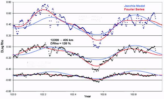 Fig. 1. Semiannual density variation for 2002 for selected satellites. Individual points
are daily density difference values. Jacchia’s model and individual satellite
Fourier fit also plotted. The top and bottom set of curves have been offset in
Dlog Rho (Δlog10ρ) by +0.5 and –0.5 respectively for clarity.
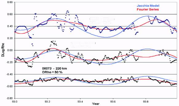 Fig. 2. Semiannual density variation for 1993 for selected satellites. Amplitude of
semiannual variation also shown as percent density changes. The top and
bottom set of curves have been offset in Dlog Rho (Δlog10ρ) by +0.5 and –0.5
respectively for clarity.
SEMIANNUAL DENSITY VARIATION FUNCTIONInitially Jacchia4 represented the semiannual density variations as a temperature variation.
However, many difficulties arose from this that could not be explained in temperature space,
so, to remove these difficulties, Jacchia eventually had to assume that the semiannual
variation was not cause by temperature, but by direct density variations. From Jacchia’s
analysis of 12 years of satellite drag data5,6 he obtained the following equations. Jacchia
represented the semiannual density variation in the form:
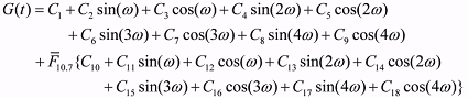
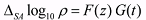 (1) (1)G(t) represents the average density variation as a function of time in which the amplitude (i.e. the difference in log10 density between the principal minimum in July and the principle
maximum in October) is normalized to 1, and F(z) is the relation between the amplitude and
the height z. Jacchia’s 197715 Model F(z) and G(t) functions are:
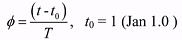
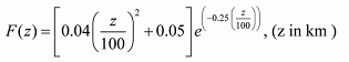 (2) (2) (3) (3)τ is a periodic function of the fraction of the tropical year T (365.0 days) corresponding to the day of the year t.
 (4) (4)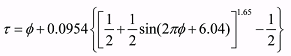 (5) (5)Other studies8 used only annual and semiannual periodic terms to capture the yearly G(t) variations, although Jacchia did not believe that using only these terms was sufficient to
capture the full semiannual variation.
In this study it was determined that a Fourier series could accurately represent Jacchia’s
G(t) equation structure and simplify the solution of the coefficients. It was determined that a
9 coefficient series, including frequencies up to 4 cycles per year, was sufficient to capture all
the variability in G(t) that had been previously observed by Jacchia and others.
It was also determined that a simplified quadratic polynomial equation in z could
sufficiently capture Jacchia’s F(z) equation and not lose any fidelity in the observed F(z) values.
The resulting equations used for the initial phase of this study were:
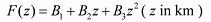 (6) (6)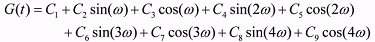 (7) (7)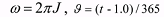 (8) (8)F(z) HEIGHT FUNCTIONThe amplitude, F(z), of the semiannual variation was determined on a year-by-year and satellite-by-satellite basis. The smoothed density difference data was fit each year for each
satellite using the 9 term Fourier series (Equation (7)). The F(z) value was then computed
from each fit as the difference between the minimum and maximum values.
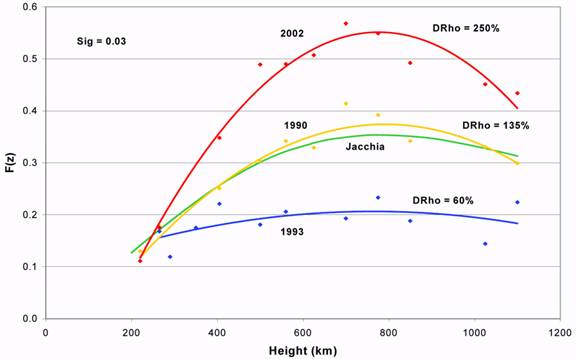 Fig. 3. The amplitude function F(z) for three different years (1990, 1993, 2002), with
semiannual amplitudes plotted for each satellite for each year. The standard
deviation, ‘sig’, of the fits is shown. The constant F(z) function from Jacchia is
also plotted.
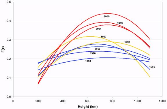 Fig. 4. The fitted F(z) curves for solar minimum (1993) through solar maximum (2001).
Solar min years are in blue, solar mid years are in yellow, and solar max years
are in red.
Figure 3 shows the results of three different years of data, along with the plot of
Jacchia’s standard 1977 F(z) equation. For each year, the
values were fit with a quadratic polynomial in height. The smoothed curves shown in Figure 3 represent the least squares quadratic fit obtained for three different years. The Δlog10ρ data for all satellites are very consistent within each year, producing a standard deviation of only 0.03. The most notable item in Figure 3 is the very large difference in maximum amplitude among the years displayed. The 2002 data shows a maximum density variation of 250% near 800km, while the 1993 data shows only a 60% maximum variation. Jacchia’s F(z) function only gives a constant 130% maximum variation for all years. Figure 4 shows the quadratic fits from solar minimum year 1993 through solar maximum year 2001. The year-to-year amplitude changes are readily apparent, with the greatest differences occurring during solar maximum. From analysis of data during the 1960s and early 1970s Jacchia found no noticeable
variation in F(z) with respect to solar activity. However, this study used over 30 years of data
covering three separate solar cycles, so an attempt was made to see if any correlation exists
between the F(z) values and the average F10.7 value. The observed maximum value of F(z) for
each year was used for the correlation. Figure 5 shows a plot of the F(z) maximum yearly
values with respect to the yearly F10.7 average. The maximum F(z) values show an extremely
high correlation with the yearly average value of F10.7. Three years, 1988, 1993, and 2002
were rejected from the fit because their values deviated by more than 3 sigma from the fitted
line shown in the figure. Some error was introduced using a yearly average of F10.7.
However, the resulting fitted sigma was 0.04 in Δlog10ρ, indicating a very good fit with high
correlation.
Figure 6 shows the correlation of the each year’s maximum F(z) value with height. The data shows that the height of the maximum value moves from the 600-700 km range during
solar minimum to the 800-900 km range during solar maximum. The 600-700 km solar
minimum range is significant in that during solar minimum the major molecular constituent
above 600 km (up to 1500 km) is helium. During solar maximum the helium boundary
moves up to about 1500 km, above which it becomes the dominant constituent. This fact will
be emphasized in a later section describing when the semiannual variation disappears above
600 km during solar minimum.
To obtain a global fit, covering all years and all heights, all F(z) values for all satellites and all years were fitted to obtained the F(z) Global Model using the following equation:
 (9) (9)where z = (perigee height/1000) (km), and F10.7 is the yearly average of F10.7.
From the linear correlation of the F(z) yearly maximum with respect to F10.7 the global equation needed to include only an additional linear function of F10.7 along with the quadratic
z functionality. A sigma of 0.048 in Δlog10ρ was obtained using a 3-sigma rejection to
eliminate outlier values. The yearly maximum global F(z) values were then computed from
Equation (9). Figure 7 shows the observed yearly maximum F(z) values and the fitted F(z)
Global Model maximum values plotted as a function of date. Also shown are the 90-day
average F10.7 values. The strong correlation of the yearly maximum F(z) values with F10.7 is readily apparent. Also apparent are the occasional odd years (i.e. 1988, 1993, and 2002) that
appear to occur less than 10% of the time. In conclusion, the high variability found in the
amplitude of the semiannual variation has been discovered to indeed be highly correlated with
solar EUV activity.
 Fig. 5. The maximum F(z) value for each year plotted as a function of the yearly
average F10.7. The standard deviation, ‘sig’, of the fit is shown, as well as the
Jacchia value. The data from the years 1990 through 2000 is highlighted (1990s
Data).
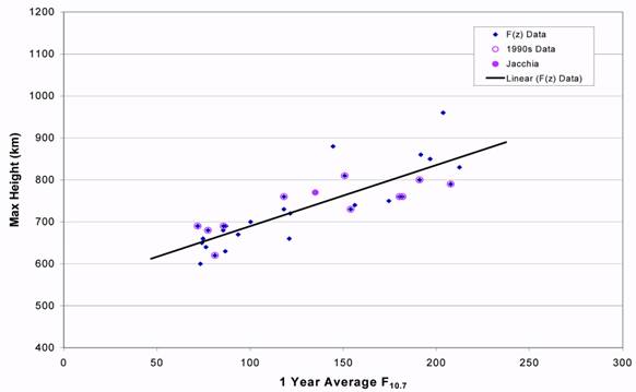 Fig. 6. The maximum F(z) value for each year plotted as a function of the height of the
maximum value. The data from the years 1990 through 2000 is highlighted
(1990s Data).
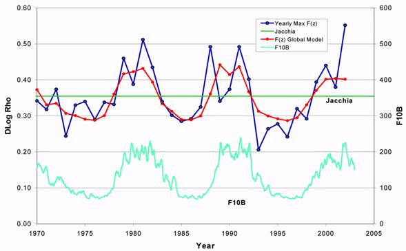 Fig. 7. The observed maximum F(z) value for each year plotted by year. Also shown
are the computed maximum F(z) values using the Global Model. The 90-day
F10.7 average, F10B, is displayed, along with Jacchia’s constant maximum
amplitude value.
G(t) YEARLY PERIODIC FUNCTIONThe G(t) function, as previously discussed, consists of a Fourier series with 9 coefficients.
The 28-day smoothed density difference data for each satellite was fitted with the Fourier
series for each year. The density difference data is the accurate observed daily density values
minus the Jacchia values without Jacchia’s semiannual variation. The G(t) function was then
obtained by normalizing to a value of 1 the difference between the minimum and maximum
values for the year. The F(z) value for each satellite by year was used for the normalization.
Figure 8 shows the results obtained for the year 1990 for the majority of the satellites. Note
the tight consistency of the curves for all heights, covering over 800 km in altitude. A yearly
G(t) function was then fit using the data for all the satellites for each year. Figure 8 also
shows the yearly G(t) value, with a standard deviation of 0.11 in Δlog10ρ. A small sigma was
obtained for every year’s fit, especially during solar maximum years. Figure 9 shows the
yearly G(t) fits for 1999 through 2001. It is readily apparent that the series changes
dramatically from year to year. During solar maximum the July minimum date can vary by as
much as 80 days. Figure 10 demonstrates the yearly G(t) variability occurring during solar
maximum and solar minimum. The variability is especially large for defining the time of the
July minimum during solar maximum, while the solar minimum times show much more
consistency from year to year.
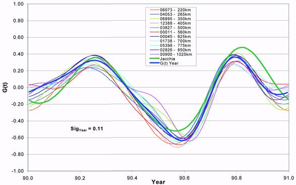 Fig. 8. The individual satellite G(t) fits are plotted for 1990. The Jacchia model and
yearly fit model are also shown. The standard deviation, ‘SigYear‘, for the G(t)
Year Model is displayed.
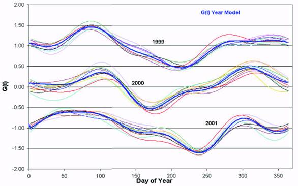 Fig. 9. The individual satellite fits for 3 different years is shown. The Year G(t) Model
is highlighted. Each set of curves for 1999 and 2001 has been offset by +1.00
and –1.00 respectively in G(t) for clarity.
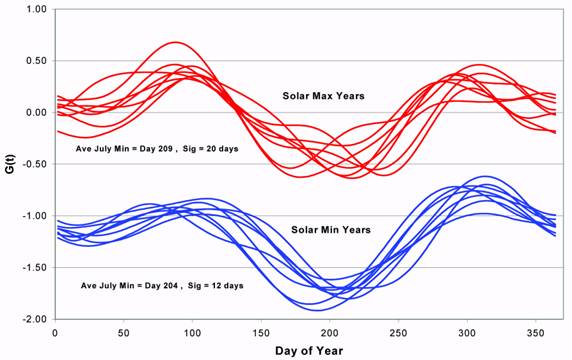 Fig. 10. The yearly G(t) fitted curves for different years are shown for solar minimum
and solar maximum conditions. The Solar Min set of curves is offset by –1.00
in G(t) for clarity. The average July minimum date with standard deviation is shown.
In an attempt to explain the variability of the July minimum date a 28-day average of
F10.7 was computed. Figure 11 shows the plots of the 28-day average, the 90-day F10.7
average, and the Year Model values, all for the year 2000. The 28-day and 90-day averages
are given for the end point of each interval. The date of a maximum difference value was
determined for each year. The maximum difference value is the maximum value of the 28-
day average above the 90-day average value occurring during the March (Day 60) through
July (Day 212) time period, always prior to the July minimum date. If there are two or more
maximums of near equal value then the closest one to the July minimum date is selected.
Figure 12 shows a plot of the date of this F10.7 maximum difference verses the date of the July
minimum for the same year. The correlation is striking. If the date of the maximum
difference occurs early in the March to July time period then the July minimum date occurs as
early as mid June. If, however, the maximum difference occurs much later in the time period
then the July minimum is delayed, sometimes to the point of occurring as late as the end of
August. It is interesting to note that other maximum differences do not appear to shift the
date of the October semiannual maximum, and they have only a small effect on shifting the
date of the semiannual April maximum. Apparently, the solar EUV is driving the phase shifts
of the semiannual July minimum as well as driving the previously shown amplitude variations
of the overall semiannual variation. This again demonstrates the need for a yearly variable
Fourier function representing the different solar conditions that occur each year.
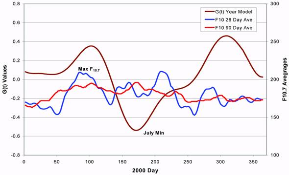 Fig. 11. Plots of the 28-day and 90-day F10.7 running averages (values are for the end point of the interval). The Year G(t) Model values are also plotted, all for the year 2000.
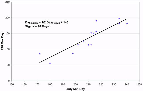 Fig. 12. The correlation of the July minimum date with the date of the F10.7 maximum
difference value. The equation for the July minimum date is given as a time lag
of the date of the F10.7 maximum difference date. Also shown is the standard
deviation, ‘Sigma’, of the linear fit.
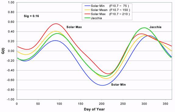 Fig. 13. The G(t) curves for different solar activity as computed from the G(t) Global
Model is shown. The standard deviation, ‘Sig’, of the global fit is displayed.
A global G(t) function was then obtained using all satellite data for all years. Since the yearly G(t) functions demonstrated a dependence on solar activity it was decided to expand
the series as a function of the 90-day average F10.7. Since the F(z) function showed only a
linear correlation with F10.7 the following equation was adopted for the global G(t) function:
 (10) (10)Figure 13 is a plot of the above global G(t) equation as fitted with all the satellite data.
Jacchia’s equation for G(t) is also shown. The standard deviation of the global fit was 0.16 Δlog10ρ. It is interesting to note that the solar minimum and solar maximum plots are significantly different except near the October maximum, which appears to have only a slight phase shift. The April maximum variation is much larger in amplitude, though not in phase.
Jacchia’s function overestimates the October maximum for all solar activity, and only
correctly estimates the April maximum during average solar activity. The curves once again
demonstrate the need for solar activity to be included in the G(t) function.
HIGH ALTITUDE SOLAR MINIMUM PHENOMENONAn interesting phenomenon occurs only during solar minimum (F10.7 < 80) at altitudes above 600 km. The following can be observed:
Figures 14 through 16, for solar minimum years 1975, 1986, and 1996, show the
occurrence of the above phenomenon. The semiannual variation has flattened out to where
there is only a hint of the October minimum. This is not the case during solar maximum
(Figures 1 and 2) where there is a significant semiannual variation at all altitudes. However,
the unmodeled 27-day variation in the density differences is still observable in Figures 14
through 16, as it is at solar maximum, with the largest variations occurring in the 600 to 700
km altitude range, and decreasing with altitude. The really interesting phenomenon that is
readily apparent is that the previously observed July minimum changes into a maximum value
as the altitude increases. At 600 to 700 km there is a hint that the July minimum is turning
into a maximum value, while at the 1100 km altitude a definite yearly July maximum is
observed. This maximum value appears to occur later and later in the year as the altitude
increases. Figure 17 shows a plot of the occurrence of the “July” minimum-maximum point
with altitude. Even with a lot of scatter in the plot it is obvious that the date of the occurrence
gets later with altitude. Below 600 km the July minimum is occurring around mid-July (year
day 190). As the altitude increases from 700 km to 1100 km the date increases from late July
to late August (year day 240). Still another interesting effect occurring during this time is the
large day-to-day scatter of density residuals. This occurs with all the satellites above 600 km,
but only during the July to late August time period. Figures 14 through 16 show the daily
density differences are smooth at all altitudes for the rest of the year except for this short time
period. The amount of scatter increases with altitude, with almost none at or below 700 km.
Satellite 00011 at 560 km showed none of the higher altitude variations in the amplitude or
scatter from the normally observed semiannual variation during solar maximum. It is as if the
atmosphere does not hold any day-to-day consistency but changes rapidly with no time
correlation. Since this is observable with all satellites, and only during this July to late
August time period, it cannot be attributed to orbit fitting problems. During solar minimum
the atmosphere is dominated by helium above 600 km (up to 1500 km), while during solar
maximum helium starts becoming dominant only above 1500 km. If the theory by Fuller-
Rowell16 is corrected (refer to the discussion below) then the atmosphere is very compressed
during the summer solstice, especially during solar minimum, which may have the effect of
replacing helium with hydrogen as the main constituent above 700 km during these time
periods. What is then being observed is the ineffectiveness of either helium or hydrogen to
retain any day-to-day correlation with solar EUV variability.
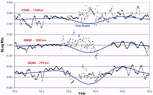 Fig. 14. Plot of Dlog Rho (Δlog10ρ) for high altitude satellites during solar minimum year 1975. The Year Model is also shown. The data and curves for 01520 and 05398
have been offset by +0.50 and –0.50 respectively for clarity.
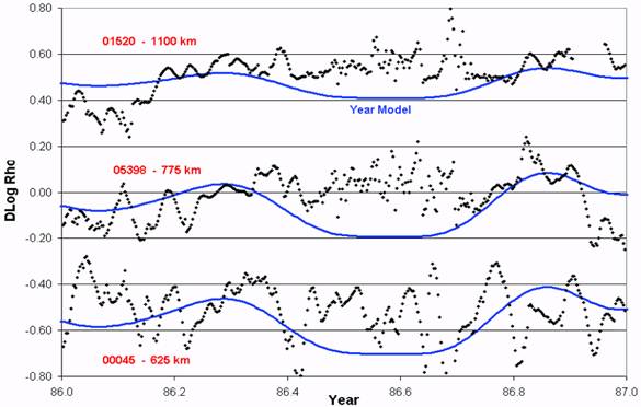 Fig. 15. Plot of Dlog Rho (Δlog10ρ) for high altitude satellites during solar minimum year 1986. The Year Model is also shown. The data and curves for 01520 and 00045
have been offset by +0.50 and –0.50 respectively for clarity.
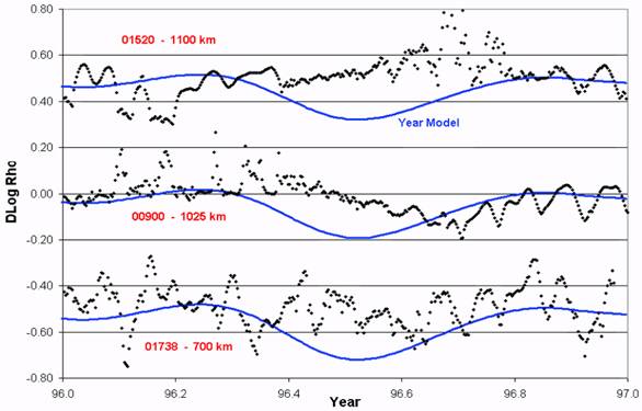 Fig. 16. Plot of Dlog Rho (Δlog10ρ) for high altitude satellites during solar minimum year 1996. The Year Model is also shown. The data and curves for 01520 and 01738
have been offset by +0.50 and –0.50 respectively for clarity.
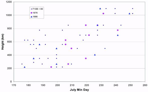 Fig. 17. The July minimum/maximum date is plotted for all satellites during solar
minimum times. The years 1976 and 1986 are highlighted.
SEMIANNUAL VARIATION DISCUSSIONIt is interesting to interpret the variation in the magnitude of the semi-annual variation with
solar activity in the context of the “thermospheric spoon” theory suggested by Fuller-
Rowell16. The “thermospheric spoon” explanation of the semi-annual variation suggests that
the global-scale, interhemispheric circulation at solstice acts like a huge turbulent eddy in
mixing the major thermospheric species. The effect causes less diffusive separation of
species at solstice, mixes the atomic and molecular neutral atmosphere species, leading to an
increase in mean mass at a given altitude. The increased mean mass at solstice reduces the
pressure scale height. The “compression” of the atmosphere leads to a reduction in the mass
density at a given height at solstice. In contrast, at equinox, the global circulation is more
symmetric and weaker. The weaker circulation no longer mixes the atmosphere, allowing the
lighter species to separate out under diffusive equilibrium. The atmosphere expands leading to
an increase in mass density at a given altitude at equinox. This theory can explain the semi-
annual variation in mass density.
Tim Fuller-Rowell17 states “the theory also suggests that the strength of the semi-annual variation is dependent on the vigor of the seasonal circulation cell. The increase in the
semiannual variation seen in the drag data therefore implies that the global circulation is
stronger at high solar activity. This is a reasonable assumption given that solar heating and
pressure gradients will be greater at solar maximum”. It remains to be seen if theoretical
physically-based models support this explanation.
SEMIANNUAL VARIATION MODEL ERROR ANALYSISAn error analysis was conducted to determine the errors of the Year, Global, and Jacchia
models previously described. The “Satellite Fit” Model was used for determining the
semiannual variation error. This model is for each individual satellite for each year fitting a 9
coefficient Fourier series to the 28-day smoothed density difference values. The fits were
done on a satellite-by-satellite basis for every year of available data. These fits should
represent the “true” year-to-year semiannual variation experienced by each satellite. The Year
Model is the year-to-year coefficients determined from all the satellites for the given year.
The Global Model is the one set of coefficients representing the semiannual variation for all
years and all altitudes. The density error from the contribution of the semiannual variation
error was obtained by differencing the Year, Global, and Jacchia models from the “Satellite
Fit” values. The total (semiannual, EUV, diurnal, etc.) error for each model was then
obtained by differencing the original density difference data from the model predictions. The
difference between the total and semiannual errors was attributed to the unmodeled EUV,
diurnal, and other density variation errors.
Figure 18 shows the semiannual density errors from the Year, Global, and Jacchia
models for solar minimum years. The Jacchia model, as expected, is the worse model, while
the Year Model is the best. The Global model appears to be modeling the semiannual
variation almost as well as the Year Model. From previous discussions the Global Model did
capture the yearly G(t) function much better at solar minimum than at solar maximum.
Figure 19 shows the semiannual density errors for all years combined. As expected the
Global Model does not show much of an improvement over the Jacchia model because of the
much larger year-to-year G(t) variations found for years with moderate to high solar activity.
However, the much lower 5-10% standard deviation for the Year Model clearly demonstrates
that a year-to-year model approach will provide a very significant reduction in the current
unmodeled semiannual density errors.
Finally, the variances of the semiannual variations are displayed in Figures 20 and 21.
The plots show that for the Jacchia model the unmodeled semiannual variations contribute to the error budget as much as the remaining unmodeled variations from EUV, diurnal, etc.
effects. Figure 21 then shows that using the Year Model greatly reduces the contribution of
the unmodeled semiannual variations, to the point that almost all of the remaining error can be
attributed to other error sources (EUV, diurnal, etc.).
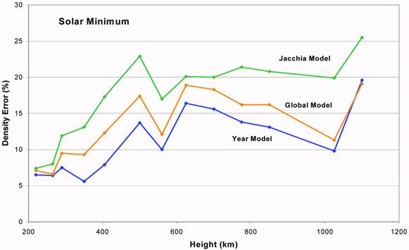 Fig. 18. The different model density errors (percent density) are shown for all data
during solar minimum periods.
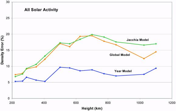 Fig. 19. The different model density errors (percent density) are shown for all data for all
solar activity.
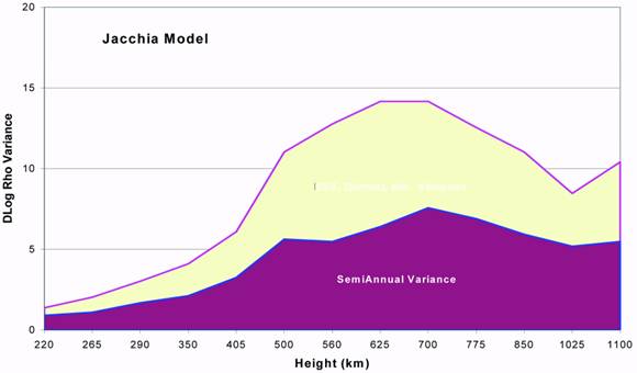 Fig. 20. The variance (times 1000) in Dlog Rho (Δlog10ρ) is shown for the semiannual errors and the remaining errors (EUV, diurnal, etc.) in the Jacchia Model.
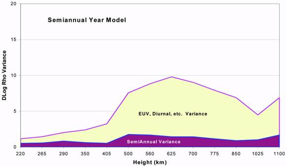 Fig. 21. The variance (times 1000) in Dlog Rho (Δlog10ρ) is shown for the semiannual errors and the remaining errors (EUV, diurnal, etc.) in the Semiannual Year
Model.
CONCLUSIONSThe following results concerning the semiannual variation have been obtained from the
current study:
Final general conclusions are:
Acknowledgments. This author would like to thank Mark Storz (USAF/AFSPC) for his insight and valuable contributions toward the theoretical development of the EDR method. The author also
thanks Tim Fuller-Rowell (NOAA/SEC) for his useful discussions and suggestions on the semiannual
density variation theory, and Robin Thurston (USAF/AFSPC) and Bill Schick (Omitron, Inc.) for
supplying the USAF Space Surveillance Network satellite observations.
REFERENCES
Размещен 29 ноября 2006.
|
|
|
|
|
|
|
|
|